Probabilities Sven Koenig, USC Russell and Norvig, 3 rd Edition, - PDF document

12/18/2019 Probabilities Sven Koenig, USC Russell and Norvig, 3 rd Edition, Chapter 13 These slides are new and can contain mistakes and typos. Please report them to Sven (skoenig@usc.edu). 1 Probabilities • Robots face lots of uncertainty. • Noisy actuators • Noisy sensors • Uncertainty in the interpretation of the sensor data • Map uncertainty • Uncertainty about their (initial) location • Uncertainty about the dynamic state of the environment [tenantsweb.org] • Probabilities can model such uncertainty. • Their semantics is well-understood. 2 1

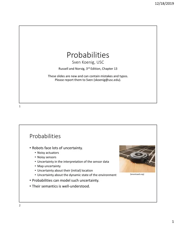
12/18/2019 Probabilities • Probability that a given random variable takes on a given value • P(random variable = value) • Example: P(number of students in class today = 68) = 0.73 • Special case that we use here: Probability that a given propositional sentence is true • P(propositional sentence) • Example: P(Sven is happy) = 0.73 3 Probabilities • What are probabilities? • Frequentist view: probabilities are frequencies in the limit (e.g. of coin flips) • Objectivist view probabilities are properties of objects (e.g. a coin) • Subjectivist view probabilities characterize the beliefs of agents • For us, probabilities are just numbers that satisfy given axioms. 4 2

12/18/2019 Probabilities • Axioms (from which one can derive how to calculate probabilities) • 0 ≤ P(A) ≤ 1 • P(true) = 1 and P(false) = 0 • P(A OR B) = P(A) + P(B) – P(A AND B) • for all propositional sentences A and B. 5 Probabilities • Examples • 1 = P(true) = P(A OR NOT A) = P(A) + P(NOT A) – P(A AND NOT A) = P(A) + P(NOT A) – P(false) = P(A) + P(NOT A) – 0 = P(A) + P(NOT A) ฀ P(NOT A) = 1 – P(A) • P(B) = P((A AND B) OR (NOT A AND B)) = P(A AND B) + P(NOT A AND B) – P((A AND B) AND (NOT A AND B)) = P(A AND B) + P(NOT A AND B) – P(false) = P(A AND B) + P(NOT A AND B) – 0 = P(A AND B) + P(NOT A AND B) (called marginalization) • P(A AND B) + P(A AND NOT B) + P(NOT A AND B) + P(NOT A AND NOT B) = (prove it yourself) = 1 • P((A AND B) OR (A AND NOT B) OR (NOT A AND B)) = (prove it yourself) = P(A AND B) + P(A AND NOT B) + P(NOT A AND B) 6 3

12/18/2019 Joint Probability Distribution • Specification of a joint probability distribution via a truth table or a Venn diagram NOT A AND NOT B A B Probability “P(A AND B)” true true P(A AND B) = 0.1 area is one sum is one true false P(A AND NOT B) = 0.2 A AND NOT B A AND B NOT A AND B false true P(NOT A AND B) = 0.2 false false P(NOT A AND NOT B) = 0.5 Sometimes we will write P(A AND B) but mean P(A AND B) for all assignments of truth values to A and B, that is, P(A AND B), P(A AND NOT B), P(NOT A AND B) and P(NOT A AND NOT B). 7 Joint Probability Distribution • Calculating probabilities • P(A OR (B EQUIV NOT A)) = P((A AND B) OR (A AND NOT B) OR (NOT A AND B)) = P(A AND B) + P(A AND NOT B) + P(NOT A AND B) = 0.1 + 0.2 + 0.2 = 0.5 A B P(A AND B) A OR (B EQUIV NOT A) NOT A AND NOT B true true P(A AND B) = 0.1 true true false P(A AND NOT B) = 0.2 true A AND NOT B A AND B NOT A AND B false true P(NOT A AND B) = 0.2 true false false P(NOT A AND NOT B) = 0.5 false • P(B) = P(A AND B) + P(NOT A AND B) = 0.1 + 0.2 = 0.3 (called marginalization) 8 4

12/18/2019 Conditional Probabilities • P(A | B) = P(A AND B) / P(B) (read: “probability of A given B”) • The probability that A is true if one knows that B is true NOT A AND NOT B • Also note: • P(A AND B) = P(A | B) P(B) = P(B | A) P(A). • P(NOT A | B) = P(NOT A AND B) / P(B) = A AND NOT B A AND B NOT A AND B (P(B) – P(A AND B)) / P(B) = P(B) / P(B) – P(A AND B) / P(B) = 1 – P(A | B). • Thus, P(A | B) + P(NOT A | B) = 1. • However, P(A | NOT B) can be any value from 0 to 1 no matter what P(A | B) is. 9 Conditional Probabilities • Calculating conditional probabilities • P(die roll = 4 | die roll = even) = 1/3 • P(die roll = 4 | die roll = odds) = 0 • P(NOT A | B) = P(NOT A AND B) / P(B) = P(NOT A AND B) / (P(A AND B) + P(NOT A AND B)) = 0.2 + (0.1 + 0.2) = 2/3 A B P(A AND B) true true P(A AND B) = 0.1 true false P(A AND NOT B) = 0.2 false true P(NOT A AND B) = 0.2 false false P(NOT A AND NOT B) = 0.5 10 5

12/18/2019 Bayes’ Rule • P(A | B) = P(A AND B) / P(B) = P(B | A) P(A) / P(B) = P(B | A) P(A) / (P(A AND B) + P(NOT A AND B)) = P(B | A) P(A) / (P(B | A) P(A) + P(B | NOT A) P(NOT A)) • P(A): prior probability (before the truth value of B is known) • P(A | B): posterior probability (after the truth value of B is known) • Example: diagnosis • P(disease | symptom) = P(symptom | disease) P(disease) / P(symptom) does often not can change over change over time time, e.g. P(flu) 11 Bayes’ Rule • You are a witness of a night-time hit-and-run accident involving a taxi in Athens. All taxis in Athens are either blue or green. You swear, under oath, that the taxis was blue. Extensive testing shows that – under the dim lighting conditions – discrimination between blue and green is 75% reliable. Calculate the most likely color for the taxi, given that 9 out of 10 Athenian taxis are green (Problem 13.21 in Russell and Norvig). 12 6

12/18/2019 Bayes’ Rule • tg = taxi was green; tb = taxi was blue; • yg = you saw a green taxi; yb = you saw a blue taxi; • P(tg) = 0.90. Thus, P(tb) = 1 – P(tg) = 1 - 0.90 = 0.10. • P(yb | tb) = 0.75. Thus, P(yg | tb) = 1 – P(yb | tb) = 1 – 0.75 = 0.25. • P(yg | tg) = 0.75. Thus, P(yb | tg) = 1 – P(yg | tg) = 1 – 0.75 = 0.25. • P(tb | yb) = P(yb | tb) P(tb) / (P(yb | tb) P(tb) + P(yb | NOT tb) P(NOT tb)) = 0.75 0.10 / (0.75 0.10 + 0.25 0.90) = 0.25. • Thus, P(tg | yb) = 1 – P(tb | yb) = 1 – 0.25 = 0.75. • Note that P(tb | yb) > P(tb) but the posterior P(tb | yb) is smaller than 0.5 since the prior P(tb) is very small. Thus, the taxi was most likely green despite your oath! 13 Independence • A and B are independent if and only if knowing the truth value of B does not change the probability that A has a given truth value, that is, (1) P(A | B) = P(A) for all assignments of truth values to A and B (that is, P(A | B) = P(A), P(NOT A | B) = P(NOT A) and so on). • Independence is symmetric since (2) P(A AND B) = P(A | B) P(B) = P(A) P(B) and (3) P(B | A) = P(A AND B) / P(A) = P(A) P(B) / P(A) = P(B) for all assignments of truth values to A and B. • One of (1), (2) or (3) can be used as the definition. The other two relationships then follow. • Example: D and N are independent for D ≡ dime lands heads and N ≡ nickel lands heads. 14 7

12/18/2019 Independence • Assume that P(A | B) = P(A). • Then, • P(NOT A | B) = 1 – P(A | B) = 1 – P(A) = P(NOT A). • P(A | B) = P(A) = P(A AND B) + P(A AND NOT B) = P(A | B) P(B) + P(A | NOT B) P(NOT B) P(A | NOT B) = P(A | B) (1 – P(B)) / P(NOT B) = P(A | B) = P(A) • P(NOT A | NOT B) = 1 – P(A | NOT B) = 1 – P(A) = P(NOT A). • Thus, P(A | B) = P(A) for all assignments of truth values to A and B. 15 Independence • Independence, when it holds, allows one to specify a joint probability distribution with fewer probabilities. • Without independence of A and B, their joint probability distribution can be specified with 3 probabilities, say P(A AND B), P(A AND NOT B) and P(NOT A AND B). Note that P(NOT A AND NOT B) = 1 – P(A AND B) – P(A AND NOT B) – P(NOT A AND B) and thus does not need to be specified. • With independence of A and B, their joint probability distribution can be specified with only 2 probabilities, say P(A) and P(B), since P(A AND B) = P(A) P(B) for all assignments of truth values to A and B. P(NOT A) = 1 – P(A) and P(NOT B) = 1 – P(B) and thus do not need to be specified. 16 8

12/18/2019 Independence • A and B are independent: A B P(A AND B) true true 0.08 = 0.4 0.2 A P(A) B P(B) true false 0.32 = 0.4 0.8 true 0.4 true 0.2 false true 0.12 = 0.6 0.2 false 0.6 false 0.8 false false 0.48 = 0.6 0.8 17 Conditional Independence • A and B are conditionally independent given C iff, when the truth value of C is known, knowing the truth value of B does not change the probability that A has a given truth value, that is, (1) P(A | B AND C) = P(A | C) for all assignments of truth values to A, B and C. • A comma is often used for an AND, e.g. P(A | B AND C) = P(A | B, C). • Similar to independence, (2) P(A, B | C) = (prove it yourself) = P(A | C) P(B| C) and (3) P(B | A, C) = (prove it yourself) = P(B | C) for all assignments of truth values to A, B and C. • One of (1), (2) or (3) can be used as the definition. The other two relationships then follow. 18 9

12/18/2019 Conditional Independence • If A and B are independent, then they are not necessarily also independent given some C. • If A and B are independent given some C, then they are not necessarily also independent. • The homework assignments are helpful to understand independence, conditional independence and their relationship better. 19 10