Review: Probabilities DISCRETE PROBABILITIES Intro We have all - PDF document

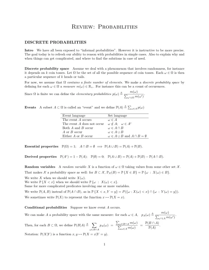
Review: Probabilities DISCRETE PROBABILITIES Intro We have all been exposed to “informal probabilities”. However it is instructive to be more precise. The goal today is to refresh our ability to reason with probabilities in simple cases. Also to explain why and when things can get complicated, and where to find the solutions in case of need. Discrete probability space Assume we deal with a phenomenon that involves randomness, for instance it depends on k coin tosses. Let Ω be the set of all the possible sequence of coin tosses. Each ω ∈ Ω is then a particular sequence of k heads or tails. For now, we assume that Ω contains a finite number of elements . We make a discrete probability space by defining for each ω ∈ Ω a measure m ( ω ) ∈ R + . For instance this can be a count of occurences. m ( ω ) ∆ Since Ω is finite we can define the elementary probabilities p ( ω ) = ω ′ ∈ Ω m ( ω ′ ). � ∆ A subset A ⊂ Ω is called an “event” and we define P ( A ) = � ω ∈ A p ( ω ) Events Event language Set language ω ∈ A The event A occurs ω ∈ A c The event A does not occur ω / ∈ A ; Both A and B occur ω ∈ A ∩ B A or B occur ω ∈ A ∪ B Either A or B occur ω ∈ A ∪ B and A ∩ B = ∅ Essential properties P (Ω) = 1; A ∩ B = ∅ = ⇒ P ( A ∪ B ) = P ( A ) + P ( B ). P ( A c ) = 1 − P ( A ); P ( ∅ ) = 0; P ( A ∪ B ) = P ( A ) + P ( B ) − P ( A ∩ B ). Derived properties A random variable X is a function of ω ∈ Ω taking values from some other set X . Random variables That makes X a probability space as well: for B ⊂ X , P X ( B ) = P { X ∈ B } = P { ω : X ( ω ) ∈ B } . We write X when we should write X ( ω ). We write P { X < x } when we should write P { ω : X ( ω ) < x } . Same for more complicated predicates involving one or more variables. We write P ( A, B ) instead of P ( A ∩ B ), as in P { X < x, Y = y } = P ( { ω : X ( ω ) < x } ∩ { ω : Y ( ω ) = y } ). We sometimes write P ( X ) to represent the function x �→ P ( X = x ). Conditional probabilities Suppose we know event A occurs. m ( ω ) ∆ We can make A a probability space with the same measure: for each ω ∈ A , p A ( ω ) = ω ′ ∈ A m ( ω ′ ). � � ω ∈ B ∩ A m ( ω ) = P ( B ∩ A ) � ∆ Then, for each B ⊂ Ω, we define P ( B | A ) = p A ( ω ) = . � ω ∈ A m ( ω ) P ( A ) ω ∈ B ∩ A Notation: P ( X | Y ) is a function x, y �→ P ( X = x | Y = y ). 1

P ( B | A ) = P ( A | B ) P ( B ) . Bayes theorem P ( A ) P ( A 1 , . . . , A n ) = P ( A 1 ) P ( A 2 | A 1 ) P ( A 3 | A 1 , A 2 ) . . . P ( A n | A 1 . . . A n − 1 ) Chain theorem Marginalization How to compute P ( A ) when one knows P ( A | X = x ) for all X ∈ X ? � � P ( A ) = P ( A, X = x ) = P ( A | X = x ) P ( X = x ) x ∈X x ∈X Events A and B are independent if knowing one tells nothing about the other. Independent events That is P ( A ) = P ( A | B ) and P ( B ) = P ( B | A ). Definition: A and B are independent iff P ( A, B ) = P ( A ) P ( B ). K � Definition: A 1 , . . . , A n are independent iff ∀ 1 ≤ i 1 < · · · < i K ≤ n, P ( A i 1 , . . . , A i K ) = P ( A i k ). k =1 This is not the same as pairwise independent: consider two coin tosses and the three events “toss 1 returns heads”, “toss 2 returns heads”, and “toss 1 and 2 return identical results”. Independent random variables ∆ X and Y are independent ⇐ ⇒ ∀ A ⊂ X , B ⊂ Y , P ( X ∈ A, Y ∈ B ) = P ( X ∈ A ) P ( Y ∈ B ). n ∆ � X 1 , . . . , X n are independent ⇐ ⇒ ∀ A 1 ⊂ X 1 , . . . , A n ⊂ X n , P ( X 1 ∈ A 1 , . . . , X n ∈ A n ) = P ( X i ∈ A i ) i =1 THE MONTY-HALL PROBLEM You are on a game show. You are given the choice of three doors: Behind one door is a car; behind the others, goats. You pick a door, say No. 1. The host, who knows where the car is, opens another door, say No. 3, and reveals a goat. He then says to you, ”Do you want to pick door No. 2?” Is it to your advantage to switch your choice? Random variables of interest The atoms are tuples ( c, m, a, h ): – c = 1 , 2 , 3 the location of the car. – m = 1 , 2 , 3 my pick of a door. – a = yes, no whether the host proposes the switch doors. – h = 1 , 2 , 3 the door picked by the host. Apply the chain rule to random variables C, M, A, H . Constructing the probability space P ( C, M, A, H ) = P ( C ) P ( M | C ) P ( A | C, M ) P ( H | C, M, A ) P ( C ) – Equiprobability: P ( C = c ) = 1 / 3. P ( M | C ) – Independence: P ( M | C ) = P ( M ) because I am not cheating. P ( A | C, M ) – Independence: P ( A | C, M ) = P ( A | M ) otherwise the host is cheating. Maybe he is. . . P ( H | C, M, A ) – This is the complicated one.  0 if h = c or h = m  P ( H = h | C = c, M = m, A = a ) = 1 / 2 if not zero and m = c if not zero and m � = c 1  2

We want P ( C | M = 1 , A = yes , H = 3 , C � = 3) = P ( C, M = 1 , A = yes , H = 3 , C � = 3) Conditionning P ( M = 1 , A = yes , H = 3 , C � = 3) We know P ( C = 1 , M = 1 , A = yes , H = 3 , C � = 3) (1 / 3) × P ( M = 1) × P ( A = yes | M = 1) × (1 / 2) = P ( C = 2 , M = 1 , A = yes , H = 3 , C � = 3) (1 / 3) × P ( M = 1) × P ( A = yes | M = 1) × 1 = P ( C = 3 , M = 1 , A = yes , H = 3 , C � = 3) = 0 Therefore P ( C = 1 | M = 1 , A = yes , H = 3 , C � = 3) = 1 / 3 P ( C = 2 | M = 1 , A = yes , H = 3 , C � = 3) = 2 / 3 P ( C = 3 | M = 1 , A = yes , H = 3 , C � = 3) = 0 What happens if the host does not know where the car is? Clueless host � 0 if h = m P ( H = h | C = c, M = m, A = a ) = 1 / 2 otherwise Then P ( C = 1 | M = 1 , A = yes , H = 3 , C � = 3) = 1 / 2 P ( C = 2 | M = 1 , A = yes , H = 3 , C � = 3) = 1 / 2 P ( C = 3 | M = 1 , A = yes , H = 3 , C � = 3) = 0 Explanation 1: The host can only reveal something he knows. Explanation 2: When c � = 1, the host has now 50% chances to open a door that reveals the car. We know he did not. Therefore the conditionning operation eliminates these cases from consideration. These cases would not have been eliminated if the host had been able to choose the right door. What happens if P ( A | C, M ) depends on C ? Cheating host – the host may decide to help us win. – the host may decide to help us loose. Reasoning Probabilities as a reasoning tool: the conclusions follow from the assumptions. Observing We could also find out whether the host is clueless or cheating by observing past instances. – If the host never reveals the car when he picks a door, he probably knows where the car is. – If the winning frequency diverges from the theoretical probabilities, I must revise my assumptions. Dual nature of probability theory is what makes it so interesting. EXPECTATION AND VARIANCE ∆ � � E [ X ] = x P ( X = x ) = X ( ω ) p ( ω ) . Expectation ω ∈ Ω x ∈X Note: we are still in the discrete case. Properties: E [1 I( A )] = P ( A ); E [ αX ] = α E [ X ]; E [ X + Y ] = E [ X ] + E [ Y ]. 3

� ∆ E [ X | Y = y ] = x P ( X = x | Y = y ) Conditional expectation x ∈X Notations: – E [ X | Y = y ] is a number. – E [ X | Y ] is a random variable that depends on the realization of Y . Properties: E [ E [ X | Y ] ] = E [ X ]. � ( X − E [ X ]) 2 � − E [ X ] 2 ∆ � X 2 � Var ( X ) = E = E Variance Properties: Var ( αX ) = α 2 Var ( X ). � Standard deviation: sdev( X ) = Var( X ). ∆ Covariance Cov( X, Y ) = E [( X − E [ X ])( Y − E [ Y ])] = E [ XY ] − E [ X ] E [ Y ] ∆ X and Y decorrelated ⇐ ⇒ Cov( X, Y ) = 0. X and Y decorrelated ⇐ ⇒ Var ( X + Y ) = Var ( X ) + Var ( Y ). X and Y decorrelated ⇐ ⇒ E [ XY ] = E [ X ] E [ Y ]. X and Y independent = ⇒ X and Y decorrelated. The converse is not necessarily true. P { X > a } ≤ E [ X ] When X is a positive real random variable, . Markov inequality a I { x > a } ≤ x/a . Proof: 1 P {| X − E [ X ] | > a } ≤ Var ( X ) . Chebyshev inequality a 2 Proof: apply Markov to ( X − E [ X ]) 2 . Interpretation: X cannot be too far from E [ X ]. Note: The a − 2 tails are not very good. – What if we apply Markov to ( X − E [ X ]) p for p greater than two ? – What if we apply Markov to e α ( X − E [ X ]) for some α positive ? The latter method leads to Chernoff bounds with exponentially small tails. Geometrical interpretation of covariances When the values of random variable X are vectors − E [ X ] E [ X ] ⊤ . ∆ � ( X − E [ X ])( X − E [ X ]) ⊤ � � X X ⊤ � Σ = E = E This is a positive symmetric matrix. Assume it is positive definite. Applying the Markov inequality to ≤ d ( X − E [ X ]) ⊤ Σ − 1 ( X − E [ X ]) ≥ a ( X − E [ X ]) ⊤ Σ − 1 ( X − E [ X ]) gives P � � a . Since ( X − E [ X ]) ⊤ Σ − 1 ( X − E [ X ]) = a is an ellipse centered on E [ X ] whose principal axes are the eigenvector of Σ and their lengths are the square root of the eigenvalues of Σ. The above result says that the data is very likely to lie inside the ellipse when a is large enough. When the ellipse if very flat, that suggests linear dependencies. 4