Comonotone lower probabilities for bivariate Introduction and - PowerPoint PPT Presentation

Comonotone lower probabilities for bivariate Introduction and discrete structures Comonotonicity for lower probabilities Building Ignacio Montes and Sebastien Destercke comonotone lower probabilities Conclusions University of Oviedo, Spain Technologic University of Compiegne, France ISIPTA 2015, July 24 1 / 17

About the authors... S. Destercke Introduction Comonotonicity for lower probabilities Building comonotone lower probabilities Conclusions https://www.hds.utc.fr/ sdesterc/dokuwiki/fr/accueil 2 / 17

About the authors... I. Montes Introduction Comonotonicity for lower probabilities Building comonotone lower probabilities Conclusions http://unimode.uniovi.es 3 / 17

Overview Introduction Introduction Comonotonicity for lower probabilities Building Comonotonicity for lower probabilities comonotone lower probabilities Conclusions Building comonotone lower probabilities Conclusions 4 / 17

Overview Introduction Introduction Comonotonicity for lower probabilities Building Comonotonicity for lower probabilities comonotone lower probabilities Conclusions Building comonotone lower probabilities Conclusions 5 / 17

Motivation Multivariate distributions take into account the dependence Introduction between the variables. Comonotonicity for lower probabilities Possible dependence between the variables: independence, Building comonotone comonotonicity, countermonotonicity, . . . lower probabilities Conclusions What happens when we have imprecise information? Independence for imprecise probabilities has already been studied. And what about comonotonicity? 6 / 17

Overview Introduction Introduction Comonotonicity for lower probabilities Building Comonotonicity for lower probabilities comonotone lower probabilities Conclusions Building comonotone lower probabilities Conclusions 7 / 17

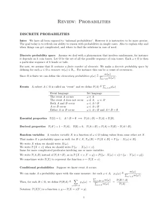
Comonotone random variables Let ( X, Y ) be a random vector defined on X × Y , and denote by P X , Y its probability distribution. P X , Y is called comonotone Introduction when the following equivalent conditions hold: Comonotonicity for lower For any ( x, y ) ∈ X × Y , either P ( X ≤ x, Y > y ) = 0 or probabilities P ( X > x, Y ≤ y ) = 0 . Building comonotone The support of P X , Y is an increasing subset of R 2 . lower probabilities F X , Y ( x, y ) = min( F X ( x ) , F Y ( y )) for any ( x, y ) . Conclusions 8 / 17

Comonotone random variables Let ( X, Y ) be a random vector defined on X × Y , and denote by P X , Y its probability distribution. P X , Y is called comonotone Introduction when the following equivalent conditions hold: Comonotonicity for lower For any ( x, y ) ∈ X × Y , either P ( X ≤ x, Y > y ) = 0 or probabilities P ( X > x, Y ≤ y ) = 0 . Building comonotone The support of P X , Y is an increasing subset of R 2 . lower probabilities F X , Y ( x, y ) = min( F X ( x ) , F Y ( y )) for any ( x, y ) . Conclusions 2 ω 1 ω 2 ω 3 ω 4 X 2 2 3 1 Y 1 2 2 1 1 1 2 3 8 / 17

Comonotone lower probabilities Assume that P : P ( X × Y ) → [0 , 1] is a lower probability mod- elling the imprecise knowledge about P X , Y . We say that P is comonotone when any P ∈ M ( P ) is comonotone. Introduction Comonotonicity for lower probabilities Building comonotone lower probabilities Conclusions 9 / 17

Comonotone lower probabilities Assume that P : P ( X × Y ) → [0 , 1] is a lower probability mod- elling the imprecise knowledge about P X , Y . We say that P is comonotone when any P ∈ M ( P ) is comonotone. Introduction Comonotonicity for lower probabilities Example: Consider X = { x 1 , x 2 } and Y = { y 1 , y 2 } ( x 1 < Building x 2 and y 1 < y 2 ). If P ( { ( x 1 , y 2 ) } ) = 0 , any P ∈ M ( P ) is comonotone lower comonotone: probabilities Conclusions y 2 y 1 x 1 x 2 9 / 17

Characterizations Comonotone lower probabilities Introduction ∀ ( x, y ) , either ✛ ✲ Comonotonicity supp( P ) is an increasing set P ( { ( u, v ) : u > x, v ≤ y } ) = 0 or for lower probabilities P ( { ( u, v ) : u ≤ x, v > y } ) = 0 . Building ■ ❅ ❅ comonotone ❅ ❘ ❅ � ✠ � ✒ lower probabilities Any P ∈ M ( P ) Conclusions is comonotone. ❄ F ( x, y ) = min( F X ( x ) , F Y ( y )) F ( x, y ) = min( F X ( x ) , F Y ( y )) . 10 / 17

Overview Introduction Introduction Comonotonicity for lower probabilities Building Comonotonicity for lower probabilities comonotone lower probabilities Conclusions Building comonotone lower probabilities Conclusions 11 / 17

Building comonotone lower probabilities Theorem Introduction Let Bel X and Bel Y be two belief function with nested focal el- Comonotonicity for lower ements. Then, it is always possible to build a joint coherent probabilities comonotone lower probability with these fixed marginals, and in Building comonotone fact, it is also a belief function with nested focal elements. lower probabilities Theorem Conclusions Let Bel X and Bel Y be two belief functions with focal sets A 1 , . . . , A n and B 1 , . . . , B n such that A i = [ a i , a i ] and B i = [ b i , b i ] are in- tervals for i = 1 , . . . , n and m X ( A i ) = m Y ( B i ) . Then, there exists a joint coherent comonotone lower probability with these fixed marginals. Furthermore, it is a belief function. 12 / 17

Example y 3 Introduction Comonotonicity y 2 for lower probabilities Building comonotone lower probabilities y 1 Conclusions x 1 x 2 x 3 m X ( { x 2 } ) = 0 . 6 , m X ( { x 1 , x 2 , x 3 } ) = 0 . 4 . m Y ( { y 1 , y 2 } ) = 0 . 2 , m Y ( { y 1 , y 2 , y 3 } ) = 0 . 8 . 13 / 17

Example y 3 Introduction Comonotonicity y 2 for lower probabilities Building comonotone lower probabilities y 1 Conclusions x 1 x 2 x 3 m X ( { x 2 } ) = 0 . 6 , m X ( { x 1 , x 2 , x 3 } ) = 0 . 4 . m Y ( { y 1 , y 2 } ) = 0 . 2 , m Y ( { y 1 , y 2 , y 3 } ) = 0 . 8 . m X ( { x 2 } ) = 0 . 2 , m X ( { x 2 } ) = 0 . 4 , m X ( { x 1 , x 2 , x 3 } ) = 0 . 4 . m Y ( { y 1 , y 2 } ) = 0 . 2 , m Y ( { y 1 , y 2 , y 3 } ) = 0 . 4 , m Y ( { y 1 , y 2 , y 3 } ) = 0 . 4 . 13 / 17

Example y 3 Introduction Comonotonicity y 2 for lower probabilities Building comonotone lower probabilities y 1 Conclusions x 1 x 2 x 3 m X ( { x 2 } ) = 0 . 6 , m X ( { x 1 , x 2 , x 3 } ) = 0 . 4 . m Y ( { y 1 , y 2 } ) = 0 . 2 , m Y ( { y 1 , y 2 , y 3 } ) = 0 . 8 . m X ( { x 2 } ) = 0 . 2 , m X ( { x 2 } ) = 0 . 4 , m X ( { x 1 , x 2 , x 3 } ) = 0 . 4 . m Y ( { y 1 , y 2 } ) = 0 . 2 , m Y ( { y 1 , y 2 , y 3 } ) = 0 . 4 , m Y ( { y 1 , y 2 , y 3 } ) = 0 . 4 . 13 / 17

Example y 3 Introduction Comonotonicity y 2 for lower probabilities Building comonotone lower probabilities y 1 Conclusions x 1 x 2 x 3 m X ( { x 2 } ) = 0 . 6 , m X ( { x 1 , x 2 , x 3 } ) = 0 . 4 . m Y ( { y 1 , y 2 } ) = 0 . 2 , m Y ( { y 1 , y 2 , y 3 } ) = 0 . 8 . m X ( { x 2 } ) = 0 . 2 , m X ( { x 2 } ) = 0 . 4 , m X ( { x 1 , x 2 , x 3 } ) = 0 . 4 . m Y ( { y 1 , y 2 } ) = 0 . 2 , m Y ( { y 1 , y 2 , y 3 } ) = 0 . 4 , m Y ( { y 1 , y 2 , y 3 } ) = 0 . 4 . 13 / 17

Example y 3 Introduction Comonotonicity y 2 for lower probabilities Building comonotone lower probabilities y 1 Conclusions x 1 x 2 x 3 m X ( { x 2 } ) = 0 . 6 , m X ( { x 1 , x 2 , x 3 } ) = 0 . 4 . m Y ( { y 1 , y 2 } ) = 0 . 2 , m Y ( { y 1 , y 2 , y 3 } ) = 0 . 8 . m X ( { x 2 } ) = 0 . 2 , m X ( { x 2 } ) = 0 . 4 , m X ( { x 1 , x 2 , x 3 } ) = 0 . 4 . m Y ( { y 1 , y 2 } ) = 0 . 2 , m Y ( { y 1 , y 2 , y 3 } ) = 0 . 4 , m Y ( { y 1 , y 2 , y 3 } ) = 0 . 4 . 13 / 17

Non-uniqueness The joint comonotone belief function may not be unique!! Introduction y 2 Comonotonicity for lower probabilities Building comonotone lower probabilities y 1 Conclusions x 1 x 2 14 / 17

Non-uniqueness The joint comonotone belief function may not be unique!! Introduction y 2 Comonotonicity for lower probabilities Building comonotone lower probabilities y 1 Conclusions x 1 x 2 14 / 17

Non-uniqueness The joint comonotone belief function may not be unique!! Introduction y 2 Comonotonicity for lower probabilities Building comonotone lower probabilities y 1 Conclusions x 1 x 2 14 / 17

Non-uniqueness The joint comonotone belief function may not be unique!! Introduction y 2 Comonotonicity for lower probabilities Building comonotone lower probabilities y 1 Conclusions x 1 x 2 14 / 17

Overview Introduction Introduction Comonotonicity for lower probabilities Building Comonotonicity for lower probabilities comonotone lower probabilities Conclusions Building comonotone lower probabilities Conclusions 15 / 17

Highlights This work investigates the notion of comonotonicity for lower Introduction probabilities. Comonotonicity for lower Definition, characterizations and properties. probabilities Building comonotone Not all marginals allow to define a joint comonotone coher- lower probabilities ent lower probability. Conclusions It does for particular cases of belief functions. Comonotonicity for bivariate p-boxes: too much restrictive. All our results can be extended to countermonotonicity. 16 / 17

Comonotone lower probabilities for bivariate Introduction and discrete structures Comonotonicity for lower probabilities Building Ignacio Montes and Sebastien Destercke comonotone lower probabilities Conclusions University of Oviedo, Spain Technologic University of Compiegne, France ISIPTA 2015, July 24 17 / 17