Bivariate and conditional distributions Edwin Leuven Today Today - PowerPoint PPT Presentation
Bivariate and conditional distributions Edwin Leuven Today Today we will continue our study of bivariate and conditional distributions Whats old (Lecture 2-4): Scatterplots, Conditional Probability, Independence Whats new:
Bivariate and conditional distributions Edwin Leuven
Today Today we will continue our study of bivariate and conditional distributions What’s old (Lecture 2-4): ◮ Scatterplots, Conditional Probability, Independence What’s new: ◮ Conditional Expectation, Law of Total Expectation ◮ Covariance, Correlation 2/40
Draws from a continuous bivariate distribution f ( y , x ) 8 6 4 2 y 0 −2 −4 −6 −3 −2 −1 0 1 2 3 x 3/40
Draws from a continuous bivariate distribution f ( y , x ) 8 6 4 2 y 0 −2 −4 E[Y|X=x] = 1 + 2x −6 −3 −2 −1 0 1 2 3 x 4/40
Bivariate discrete distribution Labor force participation (2017, 15-74-year-olds, 1000s) In Labor Force Out of Labor Force Total Men 1466 558 2024 Women 1303 638 1941 Total 2769 1196 3965 Pr(Man) = 2024 3965 ≈ 0 . 51 Pr(Man and LF) = 1466 3965 ≈ 0 . 37 Pr(LF) = ? 5/40
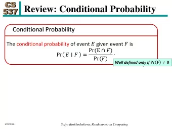
Conditional probability (Lecture 3) Pr( A | B ) = Pr( A and B ) / Pr( B ) In LF Out LF Men 1466 558 Women 1303 638 Examples: Pr(LF|Man) = 0 . 37 0 . 51 ≈ 0 . 72 Pr(LF|Woman) = 1303 1941 ≈ 0 . 67 Pr(Woman|Not LF) = ? 6/40
Conditional expectation Last week we saw that to compute the conditional expectation E [ income | men ] we simply computed the average in the conditioning group: 1 � income men = income i n men i : men This works in the same way with probabilities 7/40
Conditional expectation When Y is binary then E [ Y ] = 1 Pr( Y = 1) + 0 (1 − Pr( Y = 1)) = Pr( Y = 1) and probabilities are therefore expectations. Similarly we see that E [ Y | X ] = 1 Pr( Y = 1 | X ) + 0 (1 − Pr( Y = 1 | X )) = Pr( Y = 1 | X ) and that conditional probabilities are conditional expectations. 8/40
Conditional expectation This shows that we can compute probabilities by counting (#) occurances Pr( Y i = 1 | X i = k ) = # { Y i = 1 and X i = k } # { X i = k } and by averaging variables � � i 1 { Y i =1 , X i = k } i : X i = k 1 { Y i =1 } = 1 � Pr( Y i = 1 | X i = k ) = = Y i � i 1 { X i = k } n k n k i : X i = k where n k is the nr of observations for which X i = k , and where 1 { A } equals 1 if A is true and is 0 otherwise 9/40
Conditional expectation Remember Pr(LF|Man) = 0 . 72 Pr(LF|Woman) = 0 . 67 Pr(Man) = 0 . 51 what is Pr(LF) = ? 10/40
Conditional expectation We just applied the: Law of total expectation (iterated expectations) E [ Y ] = E X [ E [ Y | X ]] For example when X is discrete then � E [ Y ] = E [ Y | X = k ] Pr( X = k ) k when X is continuous we take the integral � E [ Y ] = E [ Y | X = x ] f ( x ) dx 11/40
Conditional expectation Note when writing E [ Y ] = E X [ E [ Y | X ]] the expectation E X just denotes that we are taking the weighted average with respect to the distribution of X For example, consider labor force participation in Norway E [LF] = E Gender [E [LF|Gender]] = E [LF|Man] Pr(Man) + E [LF|Woman] Pr(Woman) ≈ 0 . 72 × 0 . 49 + 0 . 67 × 0 . 51 ≈ 0 . 70 12/40
Conditional expectation – What is E [ Y | X = x ]? 8 6 4 2 y 0 −2 −4 −6 −3 −2 −1 0 1 2 3 x 13/40
Conditional expectation – What is E [ Y | X = x ]? - 3 : 3 ## [1] -3 -2 -1 0 1 2 3 table ( cut (x, - 3 : 3)) ## ## (-3,-2] (-2,-1] (-1,0] (0,1] (1,2] (2,3] ## 1 13 34 35 14 3 tapply (y, cut (x, - 3 : 3), mean) ## (-3,-2] (-2,-1] (-1,0] (0,1] (1,2] (2,3] ## -3.553 -1.826 0.231 1.900 3.214 5.089 The last line shows E [ Y | X ∈ ( − 3 , − 2]] = − 3 . 553 etc. 14/40
Conditional expectation – What is E [ Y | X = x ]? 8 6 4 2 y 0 −2 −4 −6 −3 −2 −1 0 1 2 3 x 15/40
Conditional expectation – What is E [ Y | X = x ]? 8 6 4 2 y 0 −2 −4 E[Y|X=x] −6 −3 −2 −1 0 1 2 3 x 16/40
Conditional variance Just like conditional expectations are subgroup averages, conditional variances Var ( Y | X ) = E [( Y − E [ Y | X ]) 2 | X ] are subgroup variances A conditional variance like Var ( income | woman ) we compute in the data as 1 � ( income i − income woman ) 2 n woman − 1 i : woman 17/40
Independence (Lecture 4) We saw that if events A and B are independent then Pr( A and B ) = Pr( A ) Pr( B ) Pr( A | B ) = Pr( A ) Similarly if two r.v.’s X and Y are independent then E [ XY ] = E [ X ] E [ Y ] E [ Y | X ] = E [ Y ] 18/40
Independence Let’s roll some independent dice iroll1 = sample (1 : 6, 1e6, replace=T) iroll2 = sample (1 : 6, 1e6, replace=T) mean (iroll1 * iroll2) ## [1] 12.2 mean (iroll1) * mean (iroll2) ## [1] 12.2 19/40
Independence Let’s roll some dependent dice droll1 = sample (1 : 6, 1e6, replace=T) droll2 = sapply (droll1, function (x) sample (1 : x, 1)) mean (droll1 * droll2) ## [1] 9.33 mean (droll1) * mean (droll2) ## [1] 7.87 20/40
Dependence We will now look at two measures that quantify dependence between random variables ◮ Covariance ◮ Correlation 21/40
Covariance The covariance quantifies the extent to which the deviation of one variable from its mean matches the deviation of another variable from its mean Cov ( X , Y ) = E [( Y − E [ Y ])( X − E [ X ])] = E [ YX − E [ X ] Y − X E [ Y ] + E [ Y ] E [ X ]] = E [ XY ] − E [ Y ] E [ X ] The covariance ◮ generalizes variance ◮ can be positive or negative ◮ equals 0 if X and Y are independent 22/40
Covariance The covariance has the following properties Cov ( X , Y ) = Cov ( Y , X ) Cov ( X , X ) = Var ( X ) Cov ( a + bX , Y ) = b Cov ( X , Y ) Cov ( X 1 + X 2 , Y ) = Cov ( X 1 , Y ) + Cov ( X 2 , Y ) 23/40
Covariance cov (iroll1, iroll2) ## [1] 0.000209 cov (droll1, droll1); var (droll1) ## [1] 2.92 ## [1] 2.92 cov (droll1, droll2) ## [1] 1.46 cov (droll1, 1 + 2 * droll2) ## [1] 2.91 24/40
Z-scores We can normalize a random variable Z = X − E [ X ] � Var ( X ) then E [ Z ] = 0 and Var ( Z ) = 1 Note that � � X − E [ X ] Var ( X ) , Y − E [ Y ] Cov ( Z X , Z Y ) = Cov � � Var ( Y ) Cov ( X , Y ) = � Var ( X ) Var ( Y ) 25/40
Correlation Pearson correlation coefficient Cov ( X , Y ) ρ ( X , Y ) = � Var ( X ) Var ( Y ) The covariance depends on the scale of the variables Correlation normalizes the covariance: ◮ − 1 ≤ ρ ( X , Y ) ≤ 1 ρ ( X , Y ) = 0 if X and Y are independent cor (droll1, droll2) ## [1] 0.617 26/40
Correlation 1 4 2 x 0 −2 −4 −4 −2 0 2 4 x <− rnorm(1000) 27/40
Correlation -1 4 2 −x 0 −2 −4 −4 −2 0 2 4 x <− rnorm(1000) 28/40
Correlation 0.5 rho * x + sqrt(1 − rho^2) * rnorm(1000) −4 −2 0 2 4 −4 −2 x <− rnorm(1000) 0 2 4 29/40
Correlation 0.7 rho * x + sqrt(1 − rho^2) * rnorm(1000) −4 −2 0 2 4 −4 −2 x <− rnorm(1000) 0 2 4 30/40
Correlation 0 4 2 rnorm(1000) 0 −2 −4 −4 −2 0 2 4 rnorm(1000) 31/40
Correlation The correlation coefficient measures the linearity between X and Y ◮ ρ ( X , Y ) = 1 then ◮ Y = a + bX with b = Var ( Y ) / Var ( X ) ◮ ρ ( X , Y ) = − 1 then ◮ Y = a + bX with b = − Var ( Y ) / Var ( X ) ◮ ρ ( X , Y ) = 0 then ◮ there is no linear relationship 32/40
Bivariate example Let Y = a + bX + U � �� � E [ Y | X ] where ◮ E [ XU ] = 0, and ◮ E [ U ] = 0 Then Cov ( X , Y ) = Cov ( X , a + bX + U ) = b Var ( X ) and therefore b = Cov ( X , Y ) Var ( X ) which shows that b is a rescaled correlation coefficient 33/40
Bivariate example Note that E [ Y ] = E [ a + bX + U ] = a + bE [ X ] + E [ U ] = a + bE [ X ] and therefore a = E [ Y ] − b E [ X ] In our data we can estimate a and b using the sample analogues � i ( x i − ¯ x )( y i − ¯ y ) b = � x ) 2 i ( x i − ¯ a = ¯ y − b ¯ x 34/40
Bivariate example plot (mydata $ x, mydata $ y, col= rgb (1,0,0,.5)) 6 4 2 mydata$y 0 −2 −2 −1 0 1 2 mydata$x 35/40
Bivariate example ## x y....1...2...x...rnorm.100. ## Min. :-2.309 Min. :-3.57 ## 1st Qu.:-0.494 1st Qu.:-0.24 ## Median : 0.062 Median : 1.21 ## Mean : 0.090 Mean : 1.07 ## 3rd Qu.: 0.692 3rd Qu.: 2.35 ## Max. : 2.187 Max. : 5.98 b = cov (mydata $ x,mydata $ y) /var (mydata $ x) a = mean (mydata $ y) - b * mean (mydata $ x) a; b ## [1] 0.897 ## [1] 1.95 36/40
Bivariate example abline (a=0.879, b=1.95) 6 4 2 mydata$y 0 −2 −2 −1 0 1 2 mydata$x 37/40
Bivariate example We have just performed a so-called ordinary least squares (OLS) regression: ## ## Call: ## lm(formula = y ~ x, data = mydata) ## ## Coefficients: ## (Intercept) x ## 0.897 1.948 38/40
Correlation is not Causation 39/40
Conclusion You understand: ◮ Bivariate distributions ◮ Conditional expectation, variance ◮ Independence ◮ Covariance ◮ Correlation You can compute and interpret ◮ conditional expectations, variances, covariances, correlations 40/40
Recommend
More recommend
Explore More Topics
Stay informed with curated content and fresh updates.
