Bivariate Correlation r > 0 r < 0 r = 0 r = 0 r > 0 r - PowerPoint PPT Presentation
Today bivariate correlation bivariate regression multiple regression Bivariate Correlation Pearson product-moment correlation (r) assesses nature and strength of the linear relationship between two continuous variables ( X
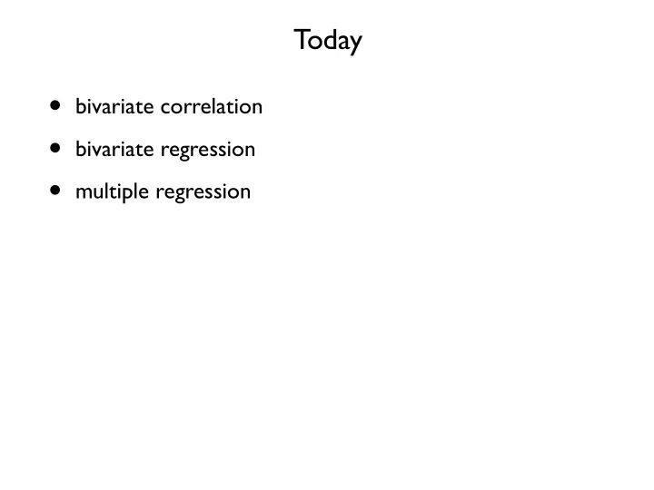
Today • bivariate correlation • bivariate regression • multiple regression
Bivariate Correlation • Pearson product-moment correlation (r) • assesses nature and strength of the linear relationship between two continuous variables � ( X − ¯ X )( Y − ¯ Y ) r = �� ( X − ¯ X ) 2 � ( Y − ¯ Y ) 2 • r^2 represents proportion of variance shared by the two variables • e.g. r=0.663, r^2=0.439: X and Y share 43.9% of the variance in common
Bivariate Correlation r > 0 r < 0 r = 0 r = 0 r > 0 r = 0 remember: r measures linear correlation
Significance Tests • we can perform significance tests on r • H0: (population) r = 0; H1: (population) r not equal to 0 (two-tailed) H1: (population) r < 0 (or >0) : one-tailed • sampling distribution of r • IF we were to randomly draw two samples from two populations that were not correlated at all, what proportion of the time would we get a value of r as as extreme as we observe? • if p < .05 we reject H0
Significance Tests F = r 2 ( N − 2) • We can perform an F-test: 1 − r 2 df = (1,N-2) • or we could also do a t-test: r t = df = N-2 � 1 − r 2 N − 2 • so for example, if we have an observed r = 0.663 based on a sample of 10 (X,Y) pairs • Fobs = 6.261 • Fcrit(1,8,0.05) = 5.32 (or compute p = 0.0368) • therefore reject H0
Significance Tests • be careful! statistical significance does not equal scientific significance • e.g. let’s say we have 112 data points we compute r = 0.2134 we do an F-test: Fobs(1,110) = 5.34, p < .05 reject H0! we have a “significant” correlation • if r=0.2134, r^2 = 0.046 only 4.6% of the variance is shared between X and Y 95.4% of the variance is NOT shared • H0 is that r = 0, not that r is large (not that r is significant )
Bivariate Regression • X, Y continuous variables • Y is considered to be dependent on X • we want to predict a value of Y, given a value of X • e.g. Y is a person’s weight, X is a person’s height ˆ Y i = β 0 + β 1 X i • estimate of Y, Yhat_i, is equal to a constant (beta_0) plus another constant (beta_1) times the value of X • this is the equation for a straight line • beta_0 is the Y-intercept, beta_1 is the slope
Bivariate Regression ˆ Y i = β 0 + β 1 X i Height Weight • we want to predict (X) (Y) Y given X 55 140 • we are modelling 61 150 Y using a linear equation 67 152 83 220 65 190 82 195 70 175 58 130 65 155 61 160
Bivariate Regression ˆ Y i = β 0 + β 1 X i Height Weight • we want to predict (X) (Y) Y given X 55 140 • we are modelling 61 150 Y using a linear equation 67 152 83 220 230 65 190 82 195 220 70 175 210 58 130 200 65 155 190 61 160 Weight Y 180 170 160 150 140 130 120 50 55 60 65 70 75 80 85 90 Height X
Bivariate Regression ˆ Y i = β 0 + β 1 X i Height Weight • we want to predict (X) (Y) Y given X 55 140 • we are modelling 61 150 Y using a linear equation 67 152 83 220 230 65 190 82 195 220 70 175 210 58 130 200 65 155 190 61 160 Weight Y 180 170 160 150 β 0 = − 7 . 2 140 130 120 50 55 60 65 70 75 80 85 90 Height X
Bivariate Regression ˆ Y i = β 0 + β 1 X i Height Weight • we want to predict (X) (Y) Y given X 55 140 • we are modelling 61 150 Y using a linear equation 67 152 83 220 230 65 190 82 195 220 70 175 210 58 130 200 65 155 190 61 160 Weight Y 180 170 160 150 β 0 = − 7 . 2 140 130 β 1 = 2 . 6 120 50 55 60 65 70 75 80 85 90 Height X
Bivariate Regression ˆ Y i = β 0 + β 1 X i Height Weight • we want to predict (X) (Y) Y given X 55 140 • we are modelling 61 150 Y using a linear equation 67 152 83 220 230 65 190 82 195 220 70 175 210 58 130 200 65 155 190 61 160 Weight Y 180 170 160 150 β 0 = − 7 . 2 140 130 β 1 = 2 . 6 120 50 55 60 65 70 75 80 85 90 Height X
Bivariate Regression ˆ Y i = β 0 + β 1 X i Height Weight (X) (Y) 55 140 61 150 67 152 83 220 230 65 190 82 195 220 70 175 210 58 130 200 65 155 190 61 160 Weight Y 180 170 160 150 β 0 = − 7 . 2 140 130 β 1 = 2 . 6 120 50 55 60 65 70 75 80 85 90 Height X
Bivariate Regression ˆ Y i = β 0 + β 1 X i Height Weight • slope means that every inch in height is (X) (Y) 55 140 associated with 2.6 pounds of weight 61 150 67 152 83 220 230 65 190 82 195 220 70 175 210 58 130 200 65 155 190 61 160 Weight Y 180 170 160 150 β 0 = − 7 . 2 140 130 β 1 = 2 . 6 120 50 55 60 65 70 75 80 85 90 Height X
Bivariate Regression • How do we estimate the coefficients beta_0 and beta_1? • for bivariate regression there are formulas: � ( X − ¯ X )( Y − ¯ Y ) β 1 = � ( X − ¯ X ) 2 β 0 = ¯ Y − β 1 ¯ X • These formulas estimate beta_0 and beta_1 according to a least-squares criterion • they are the two beta values that minimize the sum of squared deviations between the estimated values of Y (the line of best fit) and the actual values of Y (the data)
Bivariate Regression • How good is our line of best fit? • common measure is “Standard Error of Estimate” �� ( Y − ˆ Y ) 2 SE = N − 2 • N is number of (X,Y) pairs of data • SE gives a measure of the typical prediction error in units of Y • e.g. in our height/weight data • SE = sqrt(1596 / 8) = 14.1 lbs
Bivariate Regression • another measure of fit: r^2 • r^2 gives the proportion of variance accounted for • e.g. r^2 = 0.58 means that 58% of the variance in Y is accounted for by X • r^2 is bounded by [0,1] � ( ˆ Y − ¯ Y ) 2 r 2 = � ( Y − ¯ Y ) 2
Linear Regression with Non-Linear Terms Y = β 0 + β 1 X obviously non-linear relationship Y X
Linear Regression with Non-Linear Terms Y = β 0 + β 1 X 2 Y = β 0 + β 1 X obviously non-linear relationship Y X
Linear Regression with Non-Linear Terms Y = β 0 + β 1 X 2 Y = β 0 + β 1 X better but not great obviously non-linear relationship Y Y X X
Linear Regression with Non-Linear Terms Y = β 0 + β 1 X 2 Y = β 0 + β 1 X better but not great obviously non-linear relationship Y Y X X Y = β 0 + β 1 X 3
Linear Regression with Non-Linear Terms Y = β 0 + β 1 X 2 Y = β 0 + β 1 X better but not great obviously non-linear relationship Y Y X X much better fit Y = β 0 + β 1 X 3 Y X
Linear Regression with Non-Linear Terms Y = β 0 + β 1 X 3 Y • How do we do this? • Just create a new variable X^3 X • then perform linear regression using that instead of X • you will get your beta coefficients and r^2 • you can generate predicted values of Y if you want
Always plot your data • this poor fitting regression line Y = β 0 + β 1 X gives the following F-test: obviously non-linear • F(1,99)=266.2, p < .001 relationship • r^2 = 0.85 Y • so we have accounted for 85% of the variance in Y using a X straight line • is this good enough? what is H0? (y = B0) • if you never plotted the data you would never know that you can do a LOT better • with Y = B0 + B1(X^3) we get r^2 = 0.99
Always plot your data • this poor fitting regression line Y = β 0 + β 1 X gives the following F-test: obviously non-linear • F(1,99)=266.2, p < .001 relationship • r^2 = 0.85 Y • so we have accounted for 85% of the variance in Y using a X straight line • is this good enough? what is H0? (y = B0) • if you never plotted the data you would never know that you can do a LOT better • with Y = B0 + B1(X^3) we get r^2 = 0.99
Always plot your data • this poor fitting regression line Y = β 0 + β 1 X gives the following F-test: obviously non-linear • F(1,99)=266.2, p < .001 relationship • r^2 = 0.85 Y • so we have accounted for 85% of the variance in Y using a X straight line • is this good enough? what is H0? (y = B0) • if you never plotted the data you would never know that you can do a LOT better Y • with Y = B0 + B1(X^3) we get r^2 = 0.99 X
Anscombe's quartet • four datasets that have nearly identical simple statistical properties, yet appear very different when graphed • each dataset consists of eleven (x,y) points • constructed in 1973 by the statistician Francis Anscombe to demonstrate both the importance of graphing data before analyzing it and the effect of outliers on statistical properties • http://en.wikipedia.org/wiki/Anscombe's_quartet
Anscombe's quartet
Anscombe's quartet in all 4 cases: • mean(x) = 9 • var(x) = 11 • mean(y) = 7.50 • var(y) = 4.122 or 4.127 • cor(x,y) = 0.816 • regression: y = 3.00 + 0.500 (x)
Multiple Regression • same idea as bivariate regression • we want to predict values of a continuous variable Y • but instead of basing our prediction on a single variable X, • we will use several independent variables X1 .. Xk • the linear model is: ˆ Y = β 0 + β 1 X 1 + β 2 X 2 + ... + β k X k • betas are constants, X1, ..., Xk are predictor variables • beta weights are found which minimize the total sum of squared error between the predicted and actual Y values
Recommend
More recommend
Explore More Topics
Stay informed with curated content and fresh updates.
