Logistic regression to predict probabilities SU P E R VISE D L E - PowerPoint PPT Presentation

Logistic regression to predict probabilities SU P E R VISE D L E AR N IN G IN R : R E G R E SSION Nina Z u mel and John Mo u nt Win - Vector LLC

Predicting Probabilities Predicting w hether an e v ent occ u rs (y es / no ): classi � cation Predicting the probabilit y that an e v ent occ u rs : regression Linear regression : predicts v al u es in [ −∞ , ∞ ] Probabilities : limited to [0,1] inter v al So w e ' ll call it non - linear SUPERVISED LEARNING IN R : REGRESSION

E x ample : Predicting D u chenne M u sc u lar D y stroph y ( DMD ) o u tcome : has_dmd inp u ts : CK , H SUPERVISED LEARNING IN R : REGRESSION

A Linear Regression Model model <- lm(has_dmd ~ CK + H, Model predicts v al u es o u tside data = train) the range [0:1] test$pred <- predict( model, newdata = test ) o u tcome : has_dmd ∈ {0,1} 0: FALSE 1: TRUE SUPERVISED LEARNING IN R : REGRESSION

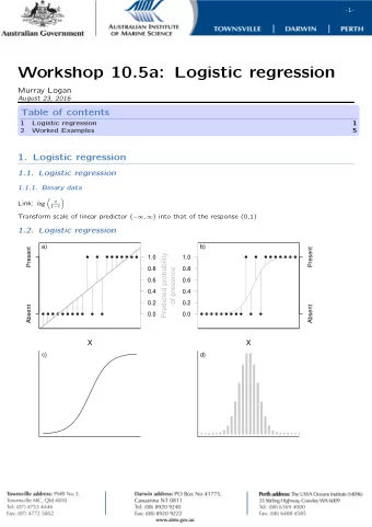
Logistic Regression p log ( ) = β + β x + β x + ... 0 1 1 2 2 1 − p glm(formula, data, family = binomial) Generali z ed linear model Ass u mes inp u ts additi v e , linear in log - odds : log ( p /(1 − p )) famil y: describes error distrib u tion of the model logistic regression : family = binomial SUPERVISED LEARNING IN R : REGRESSION

DMD model model <- glm(has_dmd ~ CK + H, data = train, family = binomial) o u tcome : t w o classes , e . g . a and b model ret u rns Prob ( b ) Recommend : 0/1 or FALSE / TRUE SUPERVISED LEARNING IN R : REGRESSION

Interpreting Logistic Regression Models model Call: glm(formula = has_dmd ~ CK + H, family = binomial, data = train) Coefficients: (Intercept) CK H -16.22046 0.07128 0.12552 Degrees of Freedom: 86 Total (i.e. Null); 84 Residual Null Deviance: 110.8 Residual Deviance: 45.16 AIC: 51.16 SUPERVISED LEARNING IN R : REGRESSION

Predicting w ith a glm () model predict(model, newdata, type = "response") newdata : b y defa u lt , training data To get probabilities : u se type = "response" B y defa u lt : ret u rns log - odds SUPERVISED LEARNING IN R : REGRESSION

DMD Model model <- glm(has_dmd ~ CK + H, data = train, family = binomial) test$pred <- predict(model, newdata = test, type = "response") SUPERVISED LEARNING IN R : REGRESSION

2 E v al u ating a logistic regression model : pse u do - R RSS 2 R = 1 − SS Tot deviance 2 pseudoR = 1 − null . deviance De v iance : analogo u s to v ariance ( RSS ) N u ll de v iance : Similar to SS Tot pse u do R ^2: De v iance e x plained SUPERVISED LEARNING IN R : REGRESSION

2 Pse u do - R on Training data Using broom::glance() glance(model) %>% + summarize(pR2 = 1 - deviance/null.deviance) pseudoR2 1 0.5922402 Using sigr::wrapChiSqTest() wrapChiSqTest(model) "... pseudo-R2=0.59 ..." SUPERVISED LEARNING IN R : REGRESSION

2 Pse u do - R on Test data # Test data test %>% + mutate(pred = predict(model, newdata = test, type = "response")) %>% + wrapChiSqTest("pred", "has_dmd", TRUE) Arg u ments : data frame prediction col u mn name o u tcome col u mn name target v al u e ( target e v ent ) SUPERVISED LEARNING IN R : REGRESSION

The Gain C u r v e Plot GainCurvePlot(test, "pred","has_dmd", "DMD model on test") SUPERVISED LEARNING IN R : REGRESSION

Let ' s practice ! SU P E R VISE D L E AR N IN G IN R : R E G R E SSION

Poisson and q u asipoisson regression to predict co u nts SU P E R VISE D L E AR N IN G IN R : R E G R E SSION Nina Z u mel and John Mo u nt Win - Vector , LLC

Predicting Co u nts Linear regression : predicts v al u es in [−∞,∞] Co u nts : integers in range [0,∞] SUPERVISED LEARNING IN R : REGRESSION

Poisson / Q u asipoisson Regression glm(formula, data, family) famil y: either poisson or quasipoisson inp u ts additi v e and linear in log ( co u nt ) SUPERVISED LEARNING IN R : REGRESSION

Poisson / Q u asipoisson Regression glm(formula, data, family) famil y: either poisson or quasipoisson inp u ts additi v e and linear in log ( co u nt ) o u tcome : integer co u nts : e . g . n u mber of tra � c tickets a dri v er gets rates : e . g . n u mber of w ebsite hits / da y prediction : e x pected rate or intensit y ( not integral ) e x pected # tra � c tickets ; e x pected hits / da y SUPERVISED LEARNING IN R : REGRESSION

Poisson v s . Q u asipoisson Poisson ass u mes that mean(y) = var(y) If var(y) m u ch di � erent from mean(y) - q u asipoisson Generall y req u ires a large sample si z e If rates / co u nts >> 0 - reg u lar regression is � ne SUPERVISED LEARNING IN R : REGRESSION

E x ample : Predicting Bike Rentals SUPERVISED LEARNING IN R : REGRESSION

Fit the model bikesJan %>% + summarize(mean = mean(cnt), var = var(cnt)) mean var 1 130.5587 14351.25 Since var(cnt) >> mean(cnt) → u se q u asipoisson fmla <- cnt ~ hr + holiday + workingday + + weathersit + temp + atemp + hum + windspeed model <- glm(fmla, data = bikesJan, family = quasipoisson) SUPERVISED LEARNING IN R : REGRESSION

Check model fit deviance 2 pseudoR = 1 − null . deviance glance(model) %>% + summarize(pseudoR2 = 1 - deviance/null.deviance) pseudoR2 1 0.7654358 SUPERVISED LEARNING IN R : REGRESSION

Predicting from the model predict(model, newdata = bikesFeb, type = "response") SUPERVISED LEARNING IN R : REGRESSION

E v al u ate the model Yo u can e v al u ate co u nt models b y RMSE bikesFeb %>% + mutate(residual = pred - cnt) %>% + summarize(rmse = sqrt(mean(residual^2))) rmse 1 69.32869 sd(bikesFeb$cnt) 134.2865 SUPERVISED LEARNING IN R : REGRESSION

Compare Predictions and Act u al O u tcomes SUPERVISED LEARNING IN R : REGRESSION

Let ' s practice ! SU P E R VISE D L E AR N IN G IN R : R E G R E SSION

GAM to learn non - linear transformations SU P E R VISE D L E AR N IN G IN R : R E G R E SSION Nina Z u mel and John Mo u nt Win - Vector , LLC

Generali z ed Additi v e Models ( GAMs ) y ∼ b 0 + s 1( x 1) + s 2( x 2) + .... SUPERVISED LEARNING IN R : REGRESSION

Learning Non - linear Relationships SUPERVISED LEARNING IN R : REGRESSION

gam () in the mgc v package gam(formula, family, data) famil y: ga u ssian ( defa u lt ): " reg u lar " regression binomial : probabilities poisson / q u asipoisson : co u nts Best for larger data sets SUPERVISED LEARNING IN R : REGRESSION

The s () f u nction anx ~ s(hassles) s() designates that v ariable sho u ld be non - linear Use s() w ith contin u o u s v ariables More than abo u t 10 u niq u e v al u es SUPERVISED LEARNING IN R : REGRESSION

Re v isit the hassles data SUPERVISED LEARNING IN R : REGRESSION

Re v isit the hassles data 2 RMSE ( cross -v al ) R ( training ) Model Linear ( hassles ) 7.69 0.53 2 Q u adratic ( hassles ) 6.89 0.63 3 C u bic ( hassles ) 6.70 0.65 SUPERVISED LEARNING IN R : REGRESSION

GAM of the hassles data model <- gam(anx ~ s(hassles), data = hassleframe, family = gaussia summary(model) ... R-sq.(adj) = 0.619 Deviance explained = 64.1% GCV = 49.132 Scale est. = 45.153 n = 40 SUPERVISED LEARNING IN R : REGRESSION

E x amining the Transformations plot(model) y v al u es : predict(model, type = "terms") SUPERVISED LEARNING IN R : REGRESSION

Predicting w ith the Model predict(model, newdata = hassleframe, type = "response") SUPERVISED LEARNING IN R : REGRESSION

Comparing o u t - of - sample performance Kno w ing the correct transformation is best , b u t GAM is u sef u l w hen transformation isn ' t kno w n 2 RMSE ( cross -v al ) R ( training ) Model Linear ( hassles ) 7.69 0.53 2 Q u adratic ( hassles ) 6.89 0.63 3 C u bic ( hassles ) 6.70 0.65 GAM 7.06 0.64 Small data set → noisier GAM SUPERVISED LEARNING IN R : REGRESSION

Let ' s practice ! SU P E R VISE D L E AR N IN G IN R : R E G R E SSION