Probabilistic PCA and Factor analysis Course of Machine Learning - PowerPoint PPT Presentation
Probabilistic PCA and Factor analysis Course of Machine Learning Master Degree in Computer Science University of Rome Tor Vergata Giorgio Gambosi a.a. 2018-2019 Idea where on a lower-dimensional subspace) lower-dimensional subspace
Probabilistic PCA and Factor analysis Course of Machine Learning Master Degree in Computer Science University of Rome “Tor Vergata” Giorgio Gambosi a.a. 2018-2019
Idea where on a lower-dimensional subspace) lower-dimensional subspace dimensions is assumed to be 0. Noise variance is assumed equal on 2 Introduce a latent variable model to relate a d -dimensional observation vector to a corresponding d ′ -dimensional gaussian latent variable (with d ′ < d ) x = Wz + µ + ϵ • z is a d ′ -dimensional gaussian latent variable (the “projection” of x • W is a d × d ′ matrix, relating the original space with the • ϵ is a d -dimensional gaussian noise: noise covariance on different all dimensions: hence p ( ϵ ) = N ( 0 , σ 2 I ) • µ is the d -dimensional vector of the means ϵ and µ are assumed independent.
Graphical model 3 σ ϵ i x i z i µ n W R d ′ , x , ϵ ∈ I R d , d ′ < d 1. z ∈ I 2. p ( z ) = N ( 0 , I ) 3. p ( ϵ ) = N ( 0 , σ 2 I ) , (isotropic gaussian noise)
Generative process This can be interpreted in terms of a generative process 4 R d ′ from 1. sample the latent variable z ∈ I 1 (2 π ) d ′ / 2 e − || z || 2 p ( z ) = 2 R d 2. linearly project onto I y = Wz + µ R d from 3. sample the noise component ϵ ∈ I (2 π ) d/ 2 e − || ϵ || 2 1 p ( ϵ ) = 2 σ 2 4. add the noise component ϵ x = y + ϵ This results into p ( x | z ) = N ( Wz + µ , σ 2 I )
Generative process 5
Probability recall Let with 6 [ ] x 1 R r R s x 1 ∈ I x 2 ∈ I x = x 2 Assume x is normally distributed: p ( x ) = N ( µ , Σ ) , and let [ ] [ ] Σ 11 Σ 12 µ 1 µ = Σ = Σ 21 Σ 22 µ 2 R r µ 1 ∈ I R s µ 2 ∈ I R r × r Σ 11 ∈ I Σ 12 = Σ T R r × s 21 ∈ I R s × s Σ 22 ∈ I
Probability recall Under the above assumptions: 7 R r , with • The marginal distribution p ( x 1 ) is a gaussian on I E [ x 1 ] = µ 1 Cov ( x 1 ) = Σ 11 R r , with • The conditional distribution p ( x 1 | x 2 ) is a gaussian on I E [ x 1 | x 2 ] = µ 1 + Σ 12 Σ − 1 22 ( x 2 − µ 2 ) Cov ( x 1 | x 2 ) = Σ 11 − Σ 12 Σ − 1 22 Σ 21
and Probability recall 8 Under the same hypotheses, the conditional distribution p ( x 1 | x 2 ) is a R r , with gaussian on I E [ x 1 | x 2 ] = µ 1 + Σ 12 Σ − 1 22 ( x 2 − µ 2 ) Cov ( x 1 | x 2 ) = Σ 11 − Σ 12 Σ − 1 22 Σ 21
Latent variable model By definition, Hence The joint distribution is 9 ([ ]) z = N ( µ zx , Σ ) p x [ ] µ z µ zx = µ x • Since p ( z ) = N ( 0 , I ) , then µ z = 0 . • Since p ( x ) = Wz + µ + ϵ , then µ x = E [ x ] = E [ Wz + µ + ϵ ] = W E [ z ] + µ + E [ ϵ ] = µ [ ] 0 µ zx = µ
Latent variable model For what concerns the distribution covariance where 10 [ ] Σ zz Σ zx Σ = Σ zx Σ xx Σ zz = E [( z − E [ z ])( z − E [ z ]) T ] = E [ zz T ] = I Σ zx = E [( z − E [ z ])( x − E [ x ]) T ] = W T Σ xx = E [( x − E [ x ])( x − E [ x ]) T ] = WW T + σ 2 I
Latent variable model Joint distribution Conditional distribution Marginal distribution 11 As a consequence, we get [ ] [ W T ] 0 I µ zx = Σ = WW T + σ 2 I W µ The marginal distribution of x is then p ( x ) = N ( µ , WW T + σ 2 I ) The conditional distribution of z given x is p ( z | x ) = N ( µ z | x , Σ z | x ) with µ z | x = W T ( WW T + σ 2 I ) − 1 ( x − µ ) Σ z | x = I − W T ( WW T + σ 2 I ) − 1 W = σ 2 ( σ 2 I + W T W ) − 1
Maximum likelihood for PCA 12 is Setting C = WW T + σ 2 I , the log-likelihood of the dataset in the model n log p ( X | W , µ , σ 2 ) = ∑ log p ( x i | W , µ , σ 2 ) i =1 n = − nd 2 log(2 π ) − n 2 log | C | − 1 ∑ ( x n − µ ) C − 1 ( x i − µ ) T 2 i =1 Setting the derivative wrt µ to zero results into n µ = x = 1 ∑ x i n i =1
Maximum likelihood for PCA solution exists: where rotation in the latent space 13 Maximization wrt W and σ 2 is more complex: however, a closed form W = U d ′ ( L d ′ − σ 2 I ) 1 / 2 R • U d ′ is the d × d ′ matrix whose columns are the eigenvectors corresponding to the d ′ largest eigenvalues • L d ′ is the d ′ × d ′ diagonal matrix of the largest eigenvalues • R is an arbitrary d ′ × d ′ orthogonal matrix, corresponding to a R can be interpreted as a rotation matrix in latent space. If R = I , the columns of W are the principal components eigenvectors scaled by the variance λ i − σ 2
Maximum likelihood for PCA since eigenvalues provide measures of the dataset variance along the corresponding eigenvector direction, this corresponds to the average variance along the discarded directions. 14 For what concerns maximization wrt σ 2 , it results d 1 σ 2 = ∑ λ i d − d ′ i = d ′ +1
Mapping points to subspace The conditional distribution can be applied. In particular, the conditional expectation 15 p ( z | x ) = N ( W T ( WW T + σ 2 I ) − 1 ( x − µ ) , σ 2 ( σ 2 I + W T W ) − 1 ) E [ z | x ] = W T ( WW T + σ 2 I ) − 1 ( x − µ ) can be assumed as the latent space point corresponding to x . The projection onto the d ′ -dimensional subspace can then be performed as x ′ = W E [ z | x ] + µ = WW T ( WW T + σ 2 I ) − 1 ( x − µ ) + µ
EM for PCA Even if the log-likelihood has a closed form maximization, applying the Expectation-Maximization algorithm can be useful in high-dimensional spaces. 16
Factor analysis Graphical model 17 variance. Noise components still gaussian and independent, but with different Ψ ϵ i x i z i µ n W R d , x , ϵ ∈ I R D , d << D 1. z ∈ I 2. p ( z ) = N ( 0 , I ) 3. p ( ϵ ) = N ( 0 , Ψ ) , Ψ diagonal (independent gaussian noise)
Factor analysis Generative model 18 R d from 1. sample the vector of factors z ∈ I (2 π ) d/ 2 exp ( − 1 1 2 || z || 2 ) p ( z ) = R D (a subspace of dimension d of 2. perform a linear projection onto I R D ) I y = Λz + µ R D from 3. sample the noise component ϵ ∈ I (2 π ) D/ 2 exp ( − 1 1 2 ϵ T Ψ − 1 ϵ ) p ( ϵ ) = 4. add the noise component ϵ x = y + ϵ
Factor analysis Model distribution are modified accordingly. 19 • Joint distribution ([ ]) ([ ] [ W T ]) z 0 I = N p , WW T + Ψ x W Λ • Marginal distribution p ( x ) = N ( µ , WW T + Ψ ) • Conditional distribution The conditional distribution of z given x is now p ( z | x ) = N ( µ z | x , Σ z | x ) with µ z | x = W T ( WW T + Ψ ) − 1 ( x − µ ) Σ z | x = I − W T ( WW T + Ψ ) − 1 W
Maximum likelihood for FA The log-likelihood of the dataset in the model is now Expecation-Maximization must be applied. Estimating parameters through log-likelihood maximization does not 20 n ∑ log p ( X | W , µ , Ψ ) = log p ( x i | W , µ , Ψ ) i =1 n 2 log | WW T + Ψ | − 1 = − nd 2 log(2 π ) − n ( x n − µ )( WW T + Ψ ) − ∑ 2 i =1 Setting the derivative wrt µ to zero results into n µ = x = 1 ∑ x i n i =1 provide a closed form solution for W and Ψ . Iterative techniques such as
Recommend
More recommend
Explore More Topics
Stay informed with curated content and fresh updates.
