1 Some Fun Facts 1.1 Useful Matrix Identities 1. inverse flip - PDF document

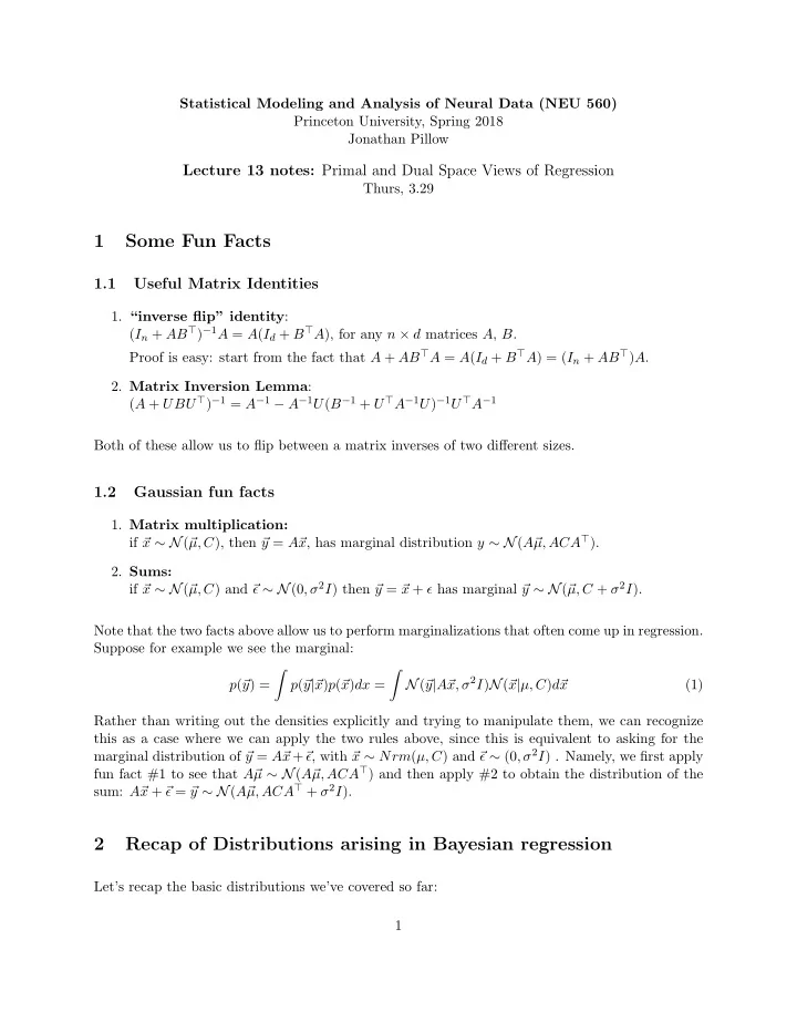
Statistical Modeling and Analysis of Neural Data (NEU 560) Princeton University, Spring 2018 Jonathan Pillow Lecture 13 notes: Primal and Dual Space Views of Regression Thurs, 3.29 1 Some Fun Facts 1.1 Useful Matrix Identities 1. “inverse flip” identity : ( I n + AB ⊤ ) − 1 A = A ( I d + B ⊤ A ), for any n × d matrices A , B . Proof is easy: start from the fact that A + AB ⊤ A = A ( I d + B ⊤ A ) = ( I n + AB ⊤ ) A . 2. Matrix Inversion Lemma : ( A + UBU ⊤ ) − 1 = A − 1 − A − 1 U ( B − 1 + U ⊤ A − 1 U ) − 1 U ⊤ A − 1 Both of these allow us to flip between a matrix inverses of two different sizes. 1.2 Gaussian fun facts 1. Matrix multiplication: µ, ACA ⊤ ). if � x ∼ N ( � µ, C ), then � y = A� x , has marginal distribution y ∼ N ( A� 2. Sums: ǫ ∼ N (0 , σ 2 I ) then � µ, C + σ 2 I ). if � x ∼ N ( � µ, C ) and � y = � x + ǫ has marginal � y ∼ N ( � Note that the two facts above allow us to perform marginalizations that often come up in regression. Suppose for example we see the marginal: � � x, σ 2 I ) N ( � p ( � y ) = p ( � y | � x ) p ( � x ) dx = N ( � y | A� x | µ, C ) d� (1) x Rather than writing out the densities explicitly and trying to manipulate them, we can recognize this as a case where we can apply the two rules above, since this is equivalent to asking for the ǫ ∼ (0 , σ 2 I ) . Namely, we first apply marginal distribution of � y = A� x + � ǫ , with � x ∼ Nrm ( µ, C ) and � µ, ACA ⊤ ) and then apply #2 to obtain the distribution of the fun fact #1 to see that A� µ ∼ N ( A� µ, ACA ⊤ + σ 2 I ). sum: A� x + � ǫ = � y ∼ N ( A� 2 Recap of Distributions arising in Bayesian regression Let’s recap the basic distributions we’ve covered so far: 1

1. prior : p ( � w ). (sometimes denoted p ( � w | θ ), to emphasize dependence on some hyperparameters θ ) w ) = � n 2. likelihood : p ( Y | X, � i =1 p ( � y i | � x i , � w ) (aka “observation model”, “encoding distribution” or “conditional” when considered over Y ): w | X, Y ) 3. posterior p ( � (from Bayes’ rule) � 4. marginal likelihood : p ( Y | X ) = p ( Y | X, � w ) p ( � w ) d� w (denominator in Bayes’ rule) � 5. posterior predictive distribution : p ( Y ∗ | X ∗ , Y, X ) = p ( Y ∗ | X ∗ , � w ) p ( � w | Y, X ) d� w . (distribution over new data Y ∗ given new stimuli X ∗ and observed data ( X, Y ) used for fitting; involves integrating over uncertainty in � w ). 3 The linear Gaussian model In the case of the linear-Gaussian model (with a zero-mean Gaussian prior over weights � w and linear observation model with additive Gaussian noise), these distributions are all Guassians we can compute analytically: 1. prior : � w ∼ N (0 , C ). w, σ 2 I d ). 2. likelihood : Y | X, � w ∼ N ( X � � σ 2 X ⊤ X + C − 1 ) − 1 � ( X ⊤ X + σ 2 C − 1 ) − 1 X ⊤ Y, ( 1 3. posterior : � w | X, Y ∼ N (can be computed by completing the square) � 0 , XCX ⊤ + σ 2 I n � 4. marginal likelihood : p ( Y | X ) = N . (see notes on marginalization using Gaussian fun facts above). 5. posterior predictive : � � X ∗ ( X ⊤ X + σ 2 C − 1 ) − 1 X ⊤ Y, X ∗ ( 1 σ 2 X ⊤ X + C − 1 ) − 1 X ⊤ ∗ + σ 2 I ∗ Y ∗ | X ∗ , Y, X ∼ N (where I ∗ is an identity matrix of size given by the number of rows (stimuli) in X ∗ ; can be derived with same marginalization tricks as the marginal likelihood). 4 Primal vs. Dual space The formulas above for posterior and posterior predictive distribution are both known as primal space or weight space formulas because all the matrices that require inverting are size d × d , where d is the dimensionality of the weights � w . An alternative is to work in the dual space or function space , which instead uses matrices of size n × n , where n is the number of stimuli. Obviously, if n > d , it makes sense to work with primal space formulas. (This is the standard case 2

in linear-Gaussian regression). However, if n < d then it makes more sense to work with dual space formuas. We will see that dual space formulas allow us to work with with infinite-dimensional feature spaces, i.e., where the effective weight vector would be (in principle) infinite. 5 Dual Space formulas for linear-Gaussian model We can use the two matrix identities given above to convert the primal space formulas to their dual space equivalents. (The first identity suffices for the means, while the latter applies to the covariances). In the following we write I n to emphasize that these are n × n identity matrices, while in the primal space formulas involved I d , the d × d identity matrix. 1. posterior : � X ⊤ ( XCX ⊤ + σ 2 I n ) − 1 Y, C − CX ⊤ ( XCX ⊤ + σ 2 I n ) − 1 XC � w | X, Y ∼ N � 2. posterior predictive : � X ∗ CX ⊤ ( XCX ⊤ + σ 2 I n ) − 1 Y, Y ∗ | X ∗ , Y, X ∼ N � ∗ − X ∗ CX ⊤ ( XCX ⊤ + σ 2 I d ) − 1 XCX ⊤ X ∗ CX ⊤ ∗ + σ 2 I ∗ 6 Gram Matrix and Kernel Functions Note that in the dual space formula for the posterior predictive distribution above, we never have to explicitly represent a matrix or vector of size d ; the non-diagonal matrices all take the form or XCX ⊤ or X ∗ CX ⊤ or XCX ⊤ , which are matrices of size n × n , n ∗ × n or n × n ∗ , respectively. If we inspect the forms of these matrices, their elements all involve inner products of pairs of stimulus points. That is, the i, j ’th element of XCX ⊤ is � XCX ⊤ � x ⊤ ij = � i C� x j (2) and similarly � X ∗ CX ⊤ � x ⊤ ij = � ∗ i C� x j (3) Let K = XCX ⊤ , which is known as the Gram matrix , consisting of the function known generally x ⊤ as the kernel function k ( · , · ) applied to all pairs of stimuli, where here k ( � x i , � x j ) = � i C� x j . Let K ∗ = X ∗ CX ⊤ denote the n ∗ × n matrix formed by applying the kernel function to all test stimuli × all training stimuli, and K ∗∗ = X ∗ CX ⊤ ∗ be the n ∗ × n ∗ matrix formed by applying the kernel to all pairs of test stimuli. Then the posterior predictive distribution above can be written much more simply as: 3

posterior predictive : � � K ∗ ( K + σ 2 I ) − 1 Y, K ∗∗ − K ∗ ( K + σ 2 I ) − 1 K ⊤ ∗ + σ 2 I ∗ Y ∗ | X ∗ , Y, X ∼ N (4) As we will see in the next lecture, these formulas allow us to perform regression for models with more complex feature spaces, even infinite dimensional feature spaces. The canonical kernel function used in Gaussian Process regression is given by: x j || 2 � −|| � x i − � � k ( � x j ) = ρ exp (5) x i , � . 2 δ 2 Although we will not give the proof explicilty, this kernel function cannot be written as φ ( � x i ) · φ ( � x j ), a dot product bbetween two finite dimensional feature vectors φ ( � x i ) and φ ( � x j ). Regression using this kernel function (often called the “Gaussian”, “radial basis function (RBF)” or “squared exponential (SE)” kernel) is therefore tantamount to nonlinear regression in an infinite dimensional weight space (making use of the dual space formulation essential!). x ⊤ Of course, if we stick to the plain old linear kernel k ( � x i , � x j ) = � i C� x j , then we are back in the (finite dimensional) world of linear regression. 4