Principal components and linear mixed models Zhou Fan Yale - PowerPoint PPT Presentation
Principal components and linear mixed models Zhou Fan Yale University, Statistics and Data Science (joint w/ Iain Johnstone, Yi Sun, Zhichao Wang) Random Matrices and Related Topics Korea Institute for Advanced Study, Seoul May 6, 2019 1/37
Principal components and linear mixed models Zhou Fan Yale University, Statistics and Data Science (joint w/ Iain Johnstone, Yi Sun, Zhichao Wang) Random Matrices and Related Topics Korea Institute for Advanced Study, Seoul May 6, 2019 1/37
Linear mixed models capture multiple “levels” of variation in data. They were introduced by R. A. Fisher in 1918 to study genetic and non-genetic components of variance in quantitative traits. 2/37
Linear mixed models capture multiple “levels” of variation in data. They were introduced by R. A. Fisher in 1918 to study genetic and non-genetic components of variance in quantitative traits. This talk will describe some applications of random matrix theory to understand spectral behavior and principal components analysis for classical covariance estimates in these models. 2/37
Outline Model and motivation Results on spectral behavior A few general tools 3/37
Model and motivation 4/37
Example: A twin study Measure p quantitative traits in n / 2 pairs of twins. For i = 1 , . . . , n / 2, model this with two “levels” of variation as Y i , 1 = α i + ε i , 1 ∈ R p Y i , 2 = α i + ε i , 2 ∈ R p 5/37
Example: A twin study Measure p quantitative traits in n / 2 pairs of twins. For i = 1 , . . . , n / 2, model this with two “levels” of variation as Y i , 1 = α i + ε i , 1 ∈ R p Y i , 2 = α i + ε i , 2 ∈ R p Here, α i ∈ R p is the shared genetic effect in the i th twin pair, and ε i , 1 , ε i , 2 ∈ R p are individual variations. 5/37
Example: A twin study Measure p quantitative traits in n / 2 pairs of twins. For i = 1 , . . . , n / 2, model this with two “levels” of variation as Y i , 1 = α i + ε i , 1 ∈ R p Y i , 2 = α i + ε i , 2 ∈ R p Here, α i ∈ R p is the shared genetic effect in the i th twin pair, and ε i , 1 , ε i , 2 ∈ R p are individual variations. Assume these are random and independent, iid iid α i ∼ N (0 , Σ A ) , ε i , j ∼ N (0 , Σ E ) 5/37
Example: A twin study Measure p quantitative traits in n / 2 pairs of twins. For i = 1 , . . . , n / 2, model this with two “levels” of variation as Y i , 1 = α i + ε i , 1 ∈ R p Y i , 2 = α i + ε i , 2 ∈ R p Here, α i ∈ R p is the shared genetic effect in the i th twin pair, and ε i , 1 , ε i , 2 ∈ R p are individual variations. Assume these are random and independent, iid iid α i ∼ N (0 , Σ A ) , ε i , j ∼ N (0 , Σ E ) Only the Y i , j ’s (not the α i ’s or ε i , j ’s) are observed. From this, we wish to separately understand Σ A and Σ E . 5/37
Example: Mutations in fruit flies [McGuigan et al ’14] ... Ancestors ... ... ... Inbreeding Offspring In inbred lines of fruit lines, how much phenotypic variation arises due to genetic mutations across the generations? 6/37
Example: Mutations in fruit flies [McGuigan et al ’14] ... Ancestors ... ... ... Inbreeding Offspring In inbred lines of fruit lines, how much phenotypic variation arises due to genetic mutations across the generations? Model traits (gene expression measurements) in the j th offspring of the i th inbred line as Y i , j = α i + ε i , j . The covariance Σ A of α i ’s is the mutational variation of interest. 6/37
Example: Genome-wide association studies In n individuals, measure: • p quantitative traits, Y ∈ R n × p • genotypes { 0 , 1 , 2 } at m SNPs, X ∈ R n × m 7/37
Example: Genome-wide association studies In n individuals, measure: • p quantitative traits, Y ∈ R n × p • genotypes { 0 , 1 , 2 } at m SNPs, X ∈ R n × m Fisher’s infinitesimal model: Y = XA + E 7/37
Example: Genome-wide association studies In n individuals, measure: • p quantitative traits, Y ∈ R n × p • genotypes { 0 , 1 , 2 } at m SNPs, X ∈ R n × m Fisher’s infinitesimal model: Y = XA + E • A ∈ R m × p has independent rows α 1 , . . . , α m . Each α i ∈ R p is the contribution of the i th SNP to the observed traits. 7/37
Example: Genome-wide association studies In n individuals, measure: • p quantitative traits, Y ∈ R n × p • genotypes { 0 , 1 , 2 } at m SNPs, X ∈ R n × m Fisher’s infinitesimal model: Y = XA + E • A ∈ R m × p has independent rows α 1 , . . . , α m . Each α i ∈ R p is the contribution of the i th SNP to the observed traits. • E ∈ R n × p has independent rows ε 1 , . . . , ε n . Each ε j ∈ R p is the residual trait variation in the j th individual. 7/37
Example: Genome-wide association studies In n individuals, measure: • p quantitative traits, Y ∈ R n × p • genotypes { 0 , 1 , 2 } at m SNPs, X ∈ R n × m Fisher’s infinitesimal model: Y = XA + E • A ∈ R m × p has independent rows α 1 , . . . , α m . Each α i ∈ R p is the contribution of the i th SNP to the observed traits. • E ∈ R n × p has independent rows ε 1 , . . . , ε n . Each ε j ∈ R p is the residual trait variation in the j th individual. The covariance Σ A of α i ’s is the (additive) genetic covariance. The relative size of Σ A to Σ E provides a measure of heritability. 7/37
The linear mixed model A general model with k levels of variation is Y = U 1 A 1 + . . . + U k A k ∈ R n × p 8/37
The linear mixed model A general model with k levels of variation is Y = U 1 A 1 + . . . + U k A k ∈ R n × p • A 1 , . . . , A k are random and unobserved, with n 1 , . . . , n k independent rows distributed as N (0 , Σ 1 ) , . . . , N (0 , Σ k ). 8/37
The linear mixed model A general model with k levels of variation is Y = U 1 A 1 + . . . + U k A k ∈ R n × p • A 1 , . . . , A k are random and unobserved, with n 1 , . . . , n k independent rows distributed as N (0 , Σ 1 ) , . . . , N (0 , Σ k ). • U 1 , . . . , U k are known, deterministic, and specified by the experimental design. E.g. for the twin study, k = 2 and 1 1 ... U 1 = , U 2 = Id 1 1 8/37
The linear mixed model A general model with k levels of variation is Y = U 1 A 1 + . . . + U k A k ∈ R n × p • A 1 , . . . , A k are random and unobserved, with n 1 , . . . , n k independent rows distributed as N (0 , Σ 1 ) , . . . , N (0 , Σ k ). • U 1 , . . . , U k are known, deterministic, and specified by the experimental design. E.g. for the twin study, k = 2 and 1 1 ... U 1 = , U 2 = Id 1 1 ( k = 1, U 1 = Id is the setting of n independent observations in R p ) 8/37
The MANOVA covariance estimator For r ∈ { 1 , . . . , k } , a classical estimator for Σ r is the MANOVA estimator. This is a matrix Σ = Y T BY . � Here, B ∈ R n × n is symmetric and chosen so that E [ � Σ] = Σ r . 9/37
The MANOVA covariance estimator For r ∈ { 1 , . . . , k } , a classical estimator for Σ r is the MANOVA estimator. This is a matrix Σ = Y T BY . � Here, B ∈ R n × n is symmetric and chosen so that E [ � Σ] = Σ r . Some examples: • For k = 1 and independent observations, we take B = 1 n I . This gives the usual sample covariance matrix � Σ = 1 n Y T Y . 9/37
The MANOVA covariance estimator For r ∈ { 1 , . . . , k } , a classical estimator for Σ r is the MANOVA estimator. This is a matrix Σ = Y T BY . � Here, B ∈ R n × n is symmetric and chosen so that E [ � Σ] = Σ r . Some examples: • For k = 1 and independent observations, we take B = 1 n I . This gives the usual sample covariance matrix � Σ = 1 n Y T Y . • For k = 2 and the twin study, we take B = 1 n ( π − π ⊥ ) where π, π ⊥ are orthogonal projections onto the column span of U 1 and its complement. 9/37
The MANOVA covariance estimator Substituting Y = � r U r A r , we may express the estimator as k k � � � H T r G T Σ = r F rs G s H s r =1 s =1 • H r ≡ Σ 1 / 2 and F rs ≡ U T r BU s are deterministic r • G r are independent and random, with i.i.d. Gaussian entries 10/37
The MANOVA covariance estimator Substituting Y = � r U r A r , we may express the estimator as k k � � � H T r G T Σ = r F rs G s H s r =1 s =1 • H r ≡ Σ 1 / 2 and F rs ≡ U T r BU s are deterministic r • G r are independent and random, with i.i.d. Gaussian entries This is the random matrix model that I’ll discuss. 10/37
The MANOVA covariance estimator Substituting Y = � r U r A r , we may express the estimator as k k � � � H T r G T Σ = r F rs G s H s r =1 s =1 • H r ≡ Σ 1 / 2 and F rs ≡ U T r BU s are deterministic r • G r are independent and random, with i.i.d. Gaussian entries This is the random matrix model that I’ll discuss. 1. What is the bulk eigenvalue distribution for large n , n 1 , . . . , n k , p ? 10/37
The MANOVA covariance estimator Substituting Y = � r U r A r , we may express the estimator as k k � � � H T r G T Σ = r F rs G s H s r =1 s =1 • H r ≡ Σ 1 / 2 and F rs ≡ U T r BU s are deterministic r • G r are independent and random, with i.i.d. Gaussian entries This is the random matrix model that I’ll discuss. 1. What is the bulk eigenvalue distribution for large n , n 1 , . . . , n k , p ? 2. What is the behavior of principal components in spiked settings? 10/37
Aside: The case of isotropic noise A simple statistical null hypothesis in this model is Σ r = σ 2 r Id for every r ∈ { 1 , . . . , k } , i.e. the distribution of every random effect is isotropic noise. 11/37
Recommend
More recommend
Explore More Topics
Stay informed with curated content and fresh updates.
