Computationally Tractable Methods for High-Dimensional Data Peter B - PowerPoint PPT Presentation
Computationally Tractable Methods for High-Dimensional Data Peter B uhlmann Seminar f ur Statistik, ETH Z urich August 2008 Riboflavin production in Bacillus Subtilis in collaboration with DSM (former Roche Vitamines) response
Computationally Tractable Methods for High-Dimensional Data Peter B¨ uhlmann Seminar f¨ ur Statistik, ETH Z¨ urich August 2008
Riboflavin production in Bacillus Subtilis in collaboration with DSM (former Roche Vitamines) response variables Y ∈ R : riboflavin production rate covariates X ∈ R p : expressions from p = 4088 genes sample size n = 72 from a “homogeneous” population of genetically engineered mutants of Bacillus Subtilis p ≫ n and Gene.960 high quality data Gene.3132 Gene.48 Gene.3033 Gene.3032 Gene.1932 Gene.3034 Gene.1358 Gene.1251 Gene.1546 Gene.3031 Gene.385 Gene.816 Gene.946 Gene.3943 Gene.1564 Gene.1273 Gene.945 Gene.943 Gene.1712 Gene.2937 Gene.942 Gene.948 Gene.535 out Gene.2928 Gene.2929 Gene.3694 Gene.447 Gene.1706 Gene.1025 Gene.3693 Gene.1223 Gene.1058 Gene.2438 Gene.2439 Gene.1885 Gene.837 Gene.3312 Gene.2360 Gene.1027 Gene.289 Gene.412 Gene.1123 Gene.1640 goal: improve riboflavin production rate of Bacillus Subtilis
statistical goal: quantify importance of genes/variables in terms of association (i.e. regression) ❀ new interesting genes which we should knock-down or enhance
my primary interest: variable selection / variable importance but many of the concepts work also for the easier problem of prediction
my primary interest: variable selection / variable importance but many of the concepts work also for the easier problem of prediction
High-dimensional data ( X 1 , Y 1 ) , . . . , ( X n , Y n ) i.i.d. or stationary X i p -dimensional predictor variable Y i response variable, e.g. Y i ∈ R or Y i ∈ { 0 , 1 } high-dimensional: p ≫ n areas of application: biology, astronomy, marketing research, text classification, econometrics, ...
High-dimensional data ( X 1 , Y 1 ) , . . . , ( X n , Y n ) i.i.d. or stationary X i p -dimensional predictor variable Y i response variable, e.g. Y i ∈ R or Y i ∈ { 0 , 1 } high-dimensional: p ≫ n areas of application: biology, astronomy, marketing research, text classification, econometrics, ...
High-dimensional linear and generalized linear models p � β j X ( j ) Y i = ( β 0 +) + ǫ i , i = 1 , . . . , n , p ≫ n i j = 1 in short: Y = X β + ǫ Y i independent , E [ Y i | X i = x ] = µ ( x ) , p � β j x ( j ) , p ≫ n η ( x ) = g ( µ ( x )) = ( β 0 +) j = 1 goal: estimation of β ◮ variable selection: A true = { j ; β j � = 0 } ◮ prediction: e.g. β T X new
We need to regularize if true β true is sparse w.r.t. ◮ � β true � 0 = number of non-zero coefficients ❀ penalize with the � · � 0 -norm: argmin β ( − 2 log-likelihood ( β ) + λ � β � 0 ) , e.g. AIC, BIC ❀ computationally infeasible if p is large (2 p sub-models) ◮ � β true � 1 = � p j = 1 | β true , j | ❀ penalize with the � · � 1 -norm, i.e. Lasso: argmin β ( − 2 log-likelihood ( β ) + λ � β � 1 ) ❀ convex optimization: computationally feasible for large p alternative approaches include: Bayesian methods for regularization ❀ computationally hard (and computation is approximate)
We need to regularize if true β true is sparse w.r.t. ◮ � β true � 0 = number of non-zero coefficients ❀ penalize with the � · � 0 -norm: argmin β ( − 2 log-likelihood ( β ) + λ � β � 0 ) , e.g. AIC, BIC ❀ computationally infeasible if p is large (2 p sub-models) ◮ � β true � 1 = � p j = 1 | β true , j | ❀ penalize with the � · � 1 -norm, i.e. Lasso: argmin β ( − 2 log-likelihood ( β ) + λ � β � 1 ) ❀ convex optimization: computationally feasible for large p alternative approaches include: Bayesian methods for regularization ❀ computationally hard (and computation is approximate)
Short review on Lasso for linear models; analogous results for GLM’s Lasso for linear models ( Tibshirani, 1996 ) β ( λ ) = argmin β ( n − 1 � Y − X β � 2 + ˆ λ � β � 1 ) ���� ���� ≥ 0 P p j = 1 | β j | ❀ convex optimization problem ◮ Lasso does variable selection some of the ˆ β j ( λ ) = 0 (because of “ ℓ 1 -geometry”) ◮ ˆ β ( λ ) is (typically) a shrunken LS-estimate
Lasso for variable selection: A ( λ ) = { j ; ˆ ˆ β j ( λ ) � = 0 } no significance testing involved computationally tractable (convex optimization only) whereas � · � 0 -norm penalty methods (AIC, BIC) are computationally infeasible (2 p sub-models)
Why the Lasso/ ℓ 1 -hype? among other things (which will be discussed later) ℓ 0 -penalty problem ℓ 1 -penalty approach approximates � �� � what we usually want consider underdetermined system of linear equations: A p × p β p × 1 = b p × 1 , rank ( A ) = m < p ℓ 0 -penalty-problem: solve for β which is sparsest w.r.t. � β � 0 i.e. “Occam’s razor” Donoho & Elad (2002), ... : if A is not too ill-conditioned (in the sense of linear dependence of sub-matrices) sparsest solution β w.r.t. � · � 0 -norm = sparsest solution β w.r.t. � · � 1 -norm � �� � amounts to a convex optimization
Why the Lasso/ ℓ 1 -hype? among other things (which will be discussed later) ℓ 0 -penalty problem ℓ 1 -penalty approach approximates � �� � what we usually want consider underdetermined system of linear equations: A p × p β p × 1 = b p × 1 , rank ( A ) = m < p ℓ 0 -penalty-problem: solve for β which is sparsest w.r.t. � β � 0 i.e. “Occam’s razor” Donoho & Elad (2002), ... : if A is not too ill-conditioned (in the sense of linear dependence of sub-matrices) sparsest solution β w.r.t. � · � 0 -norm = sparsest solution β w.r.t. � · � 1 -norm � �� � amounts to a convex optimization
and also Boosting ≈ Lasso-type methods will be useful
What else do we know from theory? assumptions: linear model Y = X β + ε (or GLM) ◮ p = p n = O ( n α ) for some α < ∞ (high-dimensional) ◮ � β � 0 = no. of non-zero β j ’s = o ( n ) (sparse) ◮ conditions on the design matrix X ensuring that design matrix doesn’t exhibit “strong linear dependence”
rate-optimality up to log ( p ) -term: under “coherence conditions” for the design matrix, and for suitable λ 2 ] ≤ C σ 2 � β � 0 log ( p n ) E [ � ˆ β ( λ ) − β � 2 n (e.g. Meinshausen & Yu, 2007 ) note: for classical situation with p = � β � 0 < n 2 ] = σ 2 p n = σ 2 � β � 0 E [ � ˆ β OLS − β � 2 n
consistent variable selection: under restrictive design conditions (i.e. “neighborhood stability”), and for suitable λ , P [ ˆ A ( λ ) = A true ] = 1 − O ( exp ( − Cn 1 − δ )) ( Meinshausen & PB, 2006 ) variable screening property: under “coherence conditions” for the design matrix (weaker than neighborhood stability), and for suitable λ P [ ˆ A ( λ ) ⊇ A true ] → 1 ( n → ∞ ) ( Meinshausen & Yu, 2007;... )
in addition: for prediction-optimal λ ∗ (and nice designs) Lasso yields too large models A ( λ ∗ ) ˆ P [ ⊇ A true ] → 1 ( n → ∞ ) � �� � | ˆ A|≤ O ( min ( n , p )) ❀ Lasso as an excellent filter/screening procedure for variable selection i.e. true model is contained in selected models from Lasso the Lasso filter is easy to use, � �� � prediction optimal tuning ”computationally efficient” and statistically accurate � �� � O ( np min ( n , p ))
in addition: for prediction-optimal λ ∗ (and nice designs) Lasso yields too large models A ( λ ∗ ) ˆ P [ ⊇ A true ] → 1 ( n → ∞ ) � �� � | ˆ A|≤ O ( min ( n , p )) ❀ Lasso as an excellent filter/screening procedure for variable selection i.e. true model is contained in selected models from Lasso the Lasso filter is easy to use, � �� � prediction optimal tuning ”computationally efficient” and statistically accurate � �� � O ( np min ( n , p ))
p eff = 3 , p = 1 ′ 000 , n = 50; 2 independent realizations Lasso Lasso 2.0 2.0 1.5 1.5 cooefficients cooefficients 1.0 1.0 0.5 0.5 0.0 0.0 0 200 400 600 800 1000 0 200 400 600 800 1000 variables variables prediction-optimal tuning 44 selected variables 36 selected variables
deletion of variables with small coefficients: Adaptive Lasso (Zou, 2006): re-weighting the penalty function p n | β j | � � ( Y i − ( X β ) i ) 2 + λ ˆ β = argmin β , | ˆ β init , j | i = 1 j = 1 ˆ β init , j from Lasso in first stage (or OLS if p < n ) � �� � Zou (2006) ❀ adaptive amount of shrinkage reduces bias of the original Lasso procedure
p eff = 3 , p = 1 ′ 000 , n = 50 same 2 independent realizations from before Adaptive Lasso Adaptive Lasso 2.0 2.0 1.5 1.5 cooefficients cooefficients 1.0 1.0 0.5 0.5 0.0 0.0 0 200 400 600 800 1000 0 200 400 600 800 1000 variables variables 13 selected variables 3 selected variables (Lasso: 44 sel. var.) (Lasso: 36 sel. var.)
adaptive Lasso (with prediction-optimal penalty) always yields sparser model fits than Lasso Motif regression for transcription factor binding sites in DNA sequences n = 1300 , p = 660 Lasso Adaptive Lasso Adaptive Lasso twice no. select. variables 91 42 28 E [( ˆ Y new − Y new ) 2 ] 0.6193 0.6230 0.6226 (similar prediction performance might be due to high noise)
Recommend
More recommend
Explore More Topics
Stay informed with curated content and fresh updates.
