Outline Scheidegger Networks Networks Scheidegger NetworksA Bonus - - PowerPoint PPT Presentation

Scheidegger Networks First return random walk References Frame 1/11

Scheidegger Networks—A Bonus Calculation

Complex Networks, Course 295A, Spring, 2008

• Prof. Peter Dodds

Department of Mathematics & Statistics University of Vermont

Licensed under the Creative Commons Attribution-NonCommercial-ShareAlike 3.0 License. Scheidegger Networks First return random walk References Frame 2/11

Outline

First return random walk References

Scheidegger Networks First return random walk References Frame 3/11

Random walks

◮ We’ve seen that Scheidegger networks have random

walk boundaries [1, 2]

◮ Determining expected shape of a ‘basin’ becomes a

problem of finding the probability that a 1-d random walk returns to the origin after t time steps

◮ We solved this with a counting argument for the

discrete random walk the preceding Complex Systems course

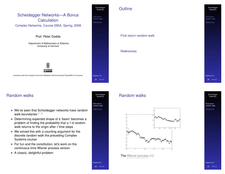
◮ For fun and the constitution, let’s work on the

continuous time Wiener process version

◮ A classic, delightful problem

Scheidegger Networks First return random walk References Frame 4/11

Random walks

The Wiener process (⊞)

Scheidegger Networks First return random walk References Frame 5/11

Random walking on a sphere...

The Wiener process (⊞)

Scheidegger Networks First return random walk References Frame 6/11

Random walks

◮ Wiener process = Brownian motion ◮

x(t2) − x(t1) ∼ N(0, t2 − t1) where N(x, t) = 1 √ 2πt e−x2/2t

◮ Continuous but nowhere differentiable

Scheidegger Networks First return random walk References Frame 7/11

First return

◮ Objective: find g(t), the probability that Wiener

process first returns to the origin at time t.

◮ Use what we know: the probability density for a

return (not necessarily the first) at time t is f(t) = 1 √ 2πt e−0/2t = 1 √ 2πt

◮ Observe that f and g are connected like this:

f(t) = t

τ=0

f(τ)g(t − τ)dτ + δ(t)

• Dirac delta function

◮ In words: Probability of returning at time t equals the

integral of the probability of returning at time τ and then not returning until exactly t − τ time units later.

Scheidegger Networks First return random walk References Frame 8/11

First return

◮ Next see that right hand side of

f(t) = t

τ=0 f(τ)g(t − τ)dτ + δ(t) is a juicy

convolution.

◮ So we take the Laplace transform:

L[f(t)] = F(s) = ∞

t=0− f(t)e−stdt ◮ and obtain

F(s) = F(s)G(s) + 1

◮ Rearrange:

G(s) = 1 − 1/F(s)

Scheidegger Networks First return random walk References Frame 9/11

First return

◮ We are here: G(s) = 1 − 1/F(s) ◮ Now we want to invert G(s) to find g(t) ◮ Use calculation that F(s) = (2s)−1/2 ◮

G(s) = 1 − (2s)1/2 ≃ e−(2s)1/2

Scheidegger Networks First return random walk References Frame 10/11

First return

Groovy aspects of g(t) ∼ t−3/2:

◮ Variance is infinite (weird but okay...) ◮ Mean is also infinite (just plain crazy...) ◮ Distribution is normalizable so process always

returns to 0.

◮ For river networks: P(ℓ) ∼ ℓ−γ so γ = 3/2 for

Scheidegger networks.

Scheidegger Networks First return random walk References Frame 11/11

References I

• A. E. Scheidegger.

A stochastic model for drainage patterns into an intramontane trench.

• Bull. Int. Assoc. Sci. Hydrol., 12(1):15–20, 1967.

.

• A. E. Scheidegger.

Theoretical Geomorphology. Springer-Verlag, New York, third edition, 1991. .