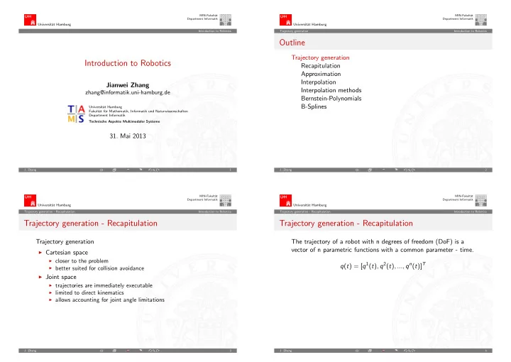
Outline Trajectory generation Introduction to Robotics - - PowerPoint PPT Presentation

Universit¨ at Hamburg

MIN-Fakult¨ at Department Informatik Introduction to Robotics

Introduction to Robotics

Jianwei Zhang

zhang@informatik.uni-hamburg.de

Universit¨ at Hamburg Fakult¨ at f¨ ur Mathematik, Informatik und Naturwissenschaften Department Informatik Technische Aspekte Multimodaler Systeme

• 31. Mai 2013
• J. Zhang

1

Universit¨ at Hamburg

MIN-Fakult¨ at Department Informatik Trajectory generation Introduction to Robotics

Outline

Trajectory generation Recapitulation Approximation Interpolation Interpolation methods Bernstein-Polynomials B-Splines

• J. Zhang

2

Universit¨ at Hamburg

MIN-Fakult¨ at Department Informatik Trajectory generation - Recapitulation Introduction to Robotics

Trajectory generation - Recapitulation

Trajectory generation

◮ Cartesian space

◮ closer to the problem ◮ better suited for collision avoidance

◮ Joint space

◮ trajectories are immediately executable ◮ limited to direct kinematics ◮ allows accounting for joint angle limitations

• J. Zhang

3

Universit¨ at Hamburg

MIN-Fakult¨ at Department Informatik Trajectory generation - Recapitulation Introduction to Robotics

Trajectory generation - Recapitulation

The trajectory of a robot with n degrees of freedom (DoF) is a vector of n parametric functions with a common parameter - time. q(t) = [q1(t), q2(t), ..., qn(t)]T

• J. Zhang

4

Universit¨ at Hamburg

MIN-Fakult¨ at Department Informatik Trajectory generation - Recapitulation Introduction to Robotics

Trajectory generation - Recapitulation

Deriving a trajectory yields

◮ 1 velocity ◮ 2 acceleration ◮ 3 jerk

Jerk represents the change of acceleration over time, allowing for non-constant accelerations. A trajectory is C k-continuous, if the first k derivations of its path exist and are continuous. A trajectory is defined as smooth if it is at least C 2-continuous.

• J. Zhang

5

Universit¨ at Hamburg

MIN-Fakult¨ at Department Informatik Trajectory generation - Approximation Introduction to Robotics

Approximation

In general, an approximation is a non-exact representation of something that is difficult to determine precisely. We are especially interested in approximating functions. Necessary if

◮ equations are hard to solve ◮ mathematically too difficult or computationally too expensive

Advantages are

◮ simple to derive ◮ simple to integrate ◮ simple to compute

• J. Zhang

6

Universit¨ at Hamburg

MIN-Fakult¨ at Department Informatik Trajectory generation - Approximation Introduction to Robotics

Approximation

Weierstrass approximation theorem (1885) was extended by Marshall Harvey Stone in 1937 to the Stone-Weierstrass theorem: For every non-periodic continuous function, there is a continuous function that can be approximated as closely as desired using algebraic polynomials. For every periodic continuous function, there is a continuous function that can be approximated as closely as desired using trigonometric polynomials.

• J. Zhang

7

Universit¨ at Hamburg

MIN-Fakult¨ at Department Informatik Trajectory generation - Interpolation Introduction to Robotics

Interpolation

Interpolation is defined as the process of constructing new data points within the range of a discrete set of known data points. Interpolation is a kind of approximation. A function is designed to match the known data points exactly, while estimating the unknown data in between in a useful way. In robotics, interpolation is especially prevalent for computing trajectories and motion/-controllers.

• J. Zhang

8

Universit¨ at Hamburg

MIN-Fakult¨ at Department Informatik Trajectory generation - Interpolation methods Introduction to Robotics

Interpolation vs. Approximation

Approximation: when a curve approximates the given data points demo: http://www.siggraph.org/education/materials/HyperGraph/modeling /splines/demoprog/curve.html Interpolation: when a curve runs exactly through all given data points In the case of many, especially noisy, data points, approximation is

• ften better suited than interpolation
• J. Zhang

9

Universit¨ at Hamburg

MIN-Fakult¨ at Department Informatik Trajectory generation - Interpolation methods Introduction to Robotics

Interpolation methods

Base is a subset of a vector space, allowing any vector in space to be uniquely represented as a finite linear combination of its members. The uniqueness of the resulting system of equations stems from the fact that polynomial of nth degree features at most n zero-points. High polynomial degrees can become difficult, as many extrema can cause oscillations. An often-used workaround is composing polynomials made of many sub-polynomials.

• J. Zhang

10

Universit¨ at Hamburg

MIN-Fakult¨ at Department Informatik Trajectory generation - Interpolation methods Introduction to Robotics

Interpolation methods

Generation of robot-trajectories in joint-space over multiple stopovers requires appropriate interpolation methods. Some interpolation methods using polynomials:

◮

Newton-polynomials

◮

Lagrange-polynomials

◮

Bernstein-polynomials

◮

Basis-Splines (B-Splines) Examples of Lagrange-polynomials and B-Splines can be found at http://www.math.ucla.edu/ baker/java/hoefer/TwoDemos.htm

• J. Zhang

11

Universit¨ at Hamburg

MIN-Fakult¨ at Department Informatik Trajectory generation - Bernstein-Polynomials Introduction to Robotics

Bernstein-Polynomials

Bernstein-polynomials (named after Sergei Natanovich Bernstein) are real polynomials with integer coefficients. Definition: Bernstein-Polynomials of degree k + 1 are defined as: Bi,k(t) = k i

• (1 − t)k−iti,

i = 0, 1, . . . , k Interpolation with Bi,k: y = b0B0,k(t) + b1B1,k(t) + · · · + bkBk,k(t)

• J. Zhang

12

Universit¨ at Hamburg

MIN-Fakult¨ at Department Informatik Trajectory generation - Bernstein-Polynomials Introduction to Robotics

Bernstein-Polynomials

Properties of Bernstein-polynomials:

◮

“basis porpety”: the Bernstein polynomials [Bi,n : 0 ≤ i ≤ n] are linearly independent and form a base of polynomial space of degree ≤ n,

◮

“decomposition of one”:

k

• i=0

Bi,k(t) ≡

k

• i=0

k

i

• ti(1 − t)k−i ≡ 1,

◮

“positivity”: Bi,k(t) ≥ 0 for t ∈ [0, 1],

◮

“recursivity”: Bi,k(t) = (1 − t)Bi,k−1(t) + t · Bi−1,k−1(t)

◮

· · ·

• J. Zhang

13

Universit¨ at Hamburg

MIN-Fakult¨ at Department Informatik Trajectory generation - Bernstein-Polynomials Introduction to Robotics

Bernstein-Polynomials

Degree 2:

• J. Zhang

14

Universit¨ at Hamburg

MIN-Fakult¨ at Department Informatik Trajectory generation - Bernstein-Polynomials Introduction to Robotics

Bernstein-Polynome

Degree 3:

• J. Zhang

15

Universit¨ at Hamburg

MIN-Fakult¨ at Department Informatik Trajectory generation - Bernstein-Polynomials Introduction to Robotics

Bernstein-Polynome

Degree 4:

Bernstein polynomials of degree 4 (cubic polynomials) are most

• ften-used, because the derivations for velocity, acceleration and jerk are

guaranteed to exist.

• J. Zhang

16

Universit¨ at Hamburg

MIN-Fakult¨ at Department Informatik Trajectory generation - B-Splines Introduction to Robotics

B-spline curves and -basis functions

A spline curve composed of B-splines is called a B-Spline curve. A B-spline curve of degree k is a polynomial composed of B-splines (basis functions) of degree k − 1 in piecewise fashion. In general, it’s k − 2 derivations are continuous at the piece’s intersections. B-splines are defined as piecewise polynomials, based on the following ordered parameters: t = (t0, t1, t2, . . . , tm, tm+1, . . . , tm+k), where

◮ m: is given by the number of points to be interpolated ◮ k: is the degree of the b-spline curve

• J. Zhang

17

Universit¨ at Hamburg

MIN-Fakult¨ at Department Informatik Trajectory generation - B-Splines Introduction to Robotics

Definition of B-splines

THe following functions are known as normalized B-splines Ni,k of

• rder k (degree k − 1):

for k = 1, Ni,k(t) = 1 : for ti ≤ t < ti+1 : else as well as a recursive definition for k > 1 Ni,k(t) = t − ti ti+k−1 − ti Ni,k−1(t)+ ti+k − t ti+k − ti+1 Ni+1,k−1(t) with i = 0, . . . , m.

• J. Zhang

18

Universit¨ at Hamburg

MIN-Fakult¨ at Department Informatik Trajectory generation - B-Splines Introduction to Robotics

B-Splines

Linear splines correspond to piecewise linear functions (squared, cubic, ...) Advantages:

◮ splines are more flexible than polynomials due to their

piecewise definition

◮ still, they are relatively simple and smooth ◮ prevents strong oscillation ◮ the values of the 1st and 2nd derivations can be selected ◮ also applicable for representing surfaces (CAD, modeling)

• J. Zhang

19

Universit¨ at Hamburg

MIN-Fakult¨ at Department Informatik Trajectory generation - B-Splines Introduction to Robotics

B-Splines

A B-spline curve can be set using so-called control-points or De-Boor-points. The curve is always constrained to those point’s convex hull. The De-Boor points are of the same dimensionality as the B-spline curve itself. B-spline curves have locality properties similar to B´ ezier-curves: the control point Pi influences the curve only within the interval [τi, τi+p]

• J. Zhang

20

Universit¨ at Hamburg

MIN-Fakult¨ at Department Informatik Trajectory generation - B-Splines Introduction to Robotics

Examples of B-splines

B-splines of degree 1, 2, 3 and 4:

• J. Zhang

21

Universit¨ at Hamburg

MIN-Fakult¨ at Department Informatik Trajectory generation - B-Splines Introduction to Robotics

Examples of B-splines

There are k overlapping B-splines within an interval An example of cubic B-splines:

• J. Zhang

22

Universit¨ at Hamburg

MIN-Fakult¨ at Department Informatik Trajectory generation - B-Splines Introduction to Robotics

B-Splines of degree k

The recursive definition of a B-spline basis function Ni,k(t):

• J. Zhang

23

Universit¨ at Hamburg

MIN-Fakult¨ at Department Informatik Trajectory generation - B-Splines Introduction to Robotics

B-splines of degree k

Segments of B-spline basis functions for degrees 2, 3 and 4 for ti ≤ t < ti+1:

• J. Zhang

24

Universit¨ at Hamburg

MIN-Fakult¨ at Department Informatik Trajectory generation - B-Splines Introduction to Robotics

Uniform B-splines of degrees 1 to 4

k=1 k=2 k=3 k=4

• J. Zhang

25

Universit¨ at Hamburg

MIN-Fakult¨ at Department Informatik Trajectory generation - B-Splines Introduction to Robotics

Uniform B-splines

◮ the distance between uniform B-splines’ control points is

constant

◮ the weight-functions of uniform B-splines are periodic ◮ this gives all functions the same form, making them easily to

compute Bk,d(u) = Bk+1,d(u+∆u) = Bk+2,d(u+2∆u), u represents the control-point’s values

• J. Zhang

26

Universit¨ at Hamburg

MIN-Fakult¨ at Department Informatik Trajectory generation - B-Splines Introduction to Robotics

Non-uniform B-splines

Degree 3:

• J. Zhang

27

Universit¨ at Hamburg

MIN-Fakult¨ at Department Informatik Trajectory generation - B-Splines Introduction to Robotics

Properties of B-splines

Partition of unity: k

i=0 Ni,k(t) = 1.

Positivity: Ni,k(t) ≥ 0. Local support: Ni,k(t) = 0 for t / ∈ [ti, ti+k]. C k−2 continuity: If the knots {ti} are pairwise different from each

• ther, then Ni,k(t) ∈ C k−2, i.e. Ni,k(t) is (k − 2) times continuously

differentiable.

• J. Zhang

28

Universit¨ at Hamburg

MIN-Fakult¨ at Department Informatik Trajectory generation - B-Splines Introduction to Robotics

Construction of a B-spline curve

A B-spline curve can be composed by combining pre-defined control-points with B-spline basis functions: r(t) =

m

• j=0

vj · Nj,k(t) where t is the position, r(t) is a point on this B-spline curve and vj are called its control points (de-Boor-Points). r(t) is a C k−2 continuous curve if the range of t is [tk−1, tm+1].

• J. Zhang

29

Universit¨ at Hamburg

MIN-Fakult¨ at Department Informatik Trajectory generation - B-Splines Introduction to Robotics

Generating control points from data points

The control points vj for interpolation are identical to the data points

• nly if k = 2.

A series of control points forms a convex hull for the interpolating curve. Two methods for generation of control points from data points: 1 by solving the following system of equations (B¨

• hm84):

qj(t) =

m

• j=0

vj · Nj,k(t) where qj are the data points to be interpolated, j = 0, · · · , m. 2 by learning, based on gradient-descend (Zhang98).

• J. Zhang

30

Universit¨ at Hamburg

MIN-Fakult¨ at Department Informatik Trajectory generation - B-Splines Introduction to Robotics

Function approximation - 1D example

A Testfunction f4(x) = 8sin(10x2 + 5x + 1) mit −1 < x < 1: the composing B-splines:

• J. Zhang

31

Universit¨ at Hamburg

MIN-Fakult¨ at Department Informatik Trajectory generation - B-Splines Introduction to Robotics

Function approximation - 2D example

Approximation of sinb(x, y) = sin(

• x2 + y 2/
• x2 + y 2)
• J. Zhang

32

Universit¨ at Hamburg

MIN-Fakult¨ at Department Informatik Trajectory generation - B-Splines Introduction to Robotics

Modelling using B-splines – examples of 3D objects

• J. Zhang

33

Universit¨ at Hamburg

MIN-Fakult¨ at Department Informatik Trajectory generation - B-Splines Introduction to Robotics

Modelling using B-splines – examples of 3D objects

• J. Zhang

34