Computer Graphics CS 543 Lecture 12 (Part 1) Curves Prof Emmanuel - PowerPoint PPT Presentation
Computer Graphics CS 543 Lecture 12 (Part 1) Curves Prof Emmanuel Agu Computer Science Dept. Worcester Polytechnic Institute (WPI) So Far Dealt with straight lines and flat surfaces Real world objects include curves Need to develop:
Computer Graphics CS 543 Lecture 12 (Part 1) Curves Prof Emmanuel Agu Computer Science Dept. Worcester Polytechnic Institute (WPI)
So Far… Dealt with straight lines and flat surfaces Real world objects include curves Need to develop: Representations of curves Tools to render curves
Curve Representation: Explicit One variable expressed in terms of another Example: z f ( x , y ) Works if one x ‐ value for each y value Example: does not work for a sphere 2 2 z x y Rarely used in CG because of this limitation
Curve Representation: Implicit Represent 2D curve or 3D surface as zeros of a formula Example: sphere representation 2 2 2 x y z 1 0 May limit classes of functions used Polynomial: function which can be expressed as linear combination of integer powers of x, y, z Degree of algebraic function: highest power in function Example: mx 4 has degree of 4
Curve Representation: Parametric Represent 2D curve as 2 functions, 1 parameter ( x ( u ), y ( u )) 3D surface as 3 functions, 2 parameters ( x ( u , v ), y ( u , v ), z ( u , v )) Example: parametric sphere x ( , ) cos cos y ( , ) cos sin z ( , ) sin
Choosing Representations Different representation suitable for different applications Implicit representations good for: Computing ray intersection with surface Determing if point is inside/outside a surface Parametric representation good for: Breaking surface into small polygonal elements for rendering Subdivide into smaller patches Sometimes possible to convert one representation into another
Continuity Consider parametric curve T P ( u ) ( x ( u ), y ( u ), z ( u )) We would like smoothest curves possible Mathematically express smoothness as continuity (no jumps) Defn: if kth derivatives exist, and are continuous, curve has kth order parametric continuity denoted C k
Continuity 0 th order means curve is continuous 1 st order means curve tangent vectors vary continuously, etc
Interactive Curve Design Mathematical formula unsuitable for designers Prefer to interactively give sequence of points (control points) Write procedure: Input: sequence of points Output: parametric representation of curve
Interactive Curve Design 1 approach: curves pass through control points (interpolate) Example: Lagrangian Interpolating Polynomial Difficulty with this approach: Polynomials always have “wiggles” For straight lines wiggling is a problem Our approach: approximate control points (Bezier, B ‐ Splines)
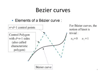
De Casteljau Algorithm Consider smooth curve that approximates sequence of control points [p0,p1,….] p ( u ) ( 1 u ) p up u 0 1 0 1 Blending functions: u and (1 – u) are non ‐ negative and sum to one
De Casteljau Algorithm Now consider 3 points 2 line segments, P0 to P1 and P1 to P2 p ( u ) ( 1 u ) p up p ( u ) ( 1 u ) p up 01 0 1 11 1 2
De Casteljau Algorithm p 01 u ( ) Substituting known values of and p 11 u ( ) p ( u ) ( 1 u ) p up ( u ) 01 11 2 2 ( 1 u ) p ( 2 u ( 1 u )) p u p 0 1 2 b 02 u ( ) b 12 u ( ) b 22 u ( ) Blending functions for degree 2 Bezier curve 2 2 b ( u ) ( 1 u ) b ( u ) u b ( u ) 2 u ( 1 u ) 02 22 12 Note: blending functions, non-negative, sum to 1
De Casteljau Algorithm Extend to 4 control points P0, P1, P2, P3 3 2 2 3 p ( u ) ( 1 u ) p ( 3 u ( 1 u ) ) p ( 3 u ( 1 u )) p u 0 1 2 b 03 u ( ) b 13 u ( ) b 23 u ( ) b 33 u ( ) Final result above is Bezier curve of degree 3
De Casteljau Algorithm 3 2 2 3 p ( u ) ( 1 u ) p ( 3 u ( 1 u ) ) p ( 3 u ( 1 u )) p u 0 1 2 b 03 u ( ) b 13 u ( ) b 23 u ( ) b 33 u ( ) Blending functions are polynomial functions called Bernstein’s polynomials 3 b ( u ) ( 1 u ) 03 2 b ( u ) 3 u ( 1 u ) 13 2 b ( u ) 3 u ( 1 u ) 23 3 b ( u ) u 33
De Casteljau Algorithm 3 2 2 3 p ( u ) ( 1 u ) p ( 3 u ( 1 u ) ) p ( 3 u ( 1 u )) p u 0 1 2 1 3 1 3 Writing coefficient of blending functions gives Pascal’s triangle 1 1 1 3 control points 1 2 1 1 4 control points 1 3 3 5 control points 1 4 6 4 1
De Casteljau Algorithm In general, blending function for k Bezier curve has form k k i i b ( u ) ( 1 u ) u ik i Example 3 3 0 0 3 b ( u ) ( 1 u ) u ( 1 u ) 03 0
De Casteljau Algorithm Can express cubic parametric curve in matrix form p 0 p 1 2 3 p ( u ) [ 1 , u , u , u ] M B p 2 p 3 where 1 0 0 0 3 3 0 0 M B 3 6 3 0 1 3 3 1
Subdividing Bezier Curves OpenGL renders flat objects To render curves, approximate with small linear segments Subdivide surface to polygonal patches Bezier curves useful for elegant, recursive subdivision
Subdividing Bezier Curves Let (P0… P3) denote original sequence of control points Recursively interpolate with u = ½ as below Sequences (P00,P01,P02,P03) and (P03,P12,P21,30) define Bezier curves also Bezier Curves can either be straightened or curved recursively in this way
Bezier Surfaces Bezier surfaces: interpolate in two dimensions This called Bilinear interpolation Example: 4 control points, P00, P01, P10, P11, 2 parameters u and v Interpolate between P00 and P01 using u P10 and P11 using u P00 and P10 using v P01 and P11 using v p ( u , v ) ( 1 v )(( 1 u ) p up ) v (( 1 u ) p up ) 00 01 10 11
Bezier Surfaces Expressing in terms of blending functions p ( u , v ) b ( v ) b ( u ) p b ( v ) b b ( u ) p b ( v ) b ( u ) p 01 01 00 01 11 01 01 11 11 11 Generalizing 3 3 p ( u , v ) b ( v ) b ( u ) p i , 3 j , 3 i , j i 0 j 0
Problems with Bezier Curves Bezier curves are elegant but too many control points To achieve smoother curve = more control points = higher order polynomial = more calculations Global support problem: All blending functions are non ‐ zero for all values of u All control points contribute to all parts of the curve Means after modelling complex surface (e.g. a ship), if one control point is moves, recalculate everything!
B ‐ Splines B ‐ splines designed to address Bezier shortcomings B ‐ Spline given by blending control points Local support: Each spline contributes in limited range Only non ‐ zero splines contribute in a given range of u m p ( u ) B ( u ) p i i i 0 B-spline blending functions, order 2
NURBS Encompasses both Bezier curves/surfaces and B ‐ splines Non ‐ uniform Rational B ‐ splines (NURBS) Rational function is ratio of two polynomials Some curves can be expressed as rational functions but not as simple polynomials No known exact polynomial for circle Rational parametrization of unit circle on xy ‐ plane: 2 1 u x ( u ) 2 1 u 2 u y ( u ) 2 1 u z ( u ) 0
NURBS We can apply homogeneous coordinates to bring in w 2 x ( u ) 1 u y ( u ) 2 u z ( u ) 0 2 w ( u ) 1 u Using w, we get we cleanly integrate rational parametrization Useful property of NURBS: preserved under transformation
Tesselation tesselation Far = Less detailed Near = More detailed mesh mesh Simplification Previously: Pre ‐ generate mesh versions offline Tesselation shader unit new to GPU in DirectX 10 (2007) Subdivide faces to yield finer detail, generate new vertices, primitives Mesh simplification/tesselation on GPU = Real time LoD Tesselation: Demo
Tessellation Shaders Can subdivide curves, surfaces on the GPU
Where Does Tesselation Shader Fit? Fixed number of vertices in/out Can change number of vertices
Step 1: Application Code Tesselation shader can generate new primitive called a patch User ‐ defined number of vertices per patch In application, use glPatchParameteri set number of vertices per patch Example: 2 patches, each with 4 vertices 8 vertices total, 4 vertices per patch
Step 2: Tessellation Control Shader Generates output vertices Sometimes pass ‐ through: same no. of vertices as input Set how much each patch should be tessellated Outer: how many segments exterior edges broken into Inner: How many inner regions (horizontal & vertical)
Recommend
More recommend
Explore More Topics
Stay informed with curated content and fresh updates.

