Outline Inference in Bayes Nets Variable Elimination Bayes Nets - PDF document
Outline Inference in Bayes Nets Variable Elimination Bayes Nets (cont) CS 486/686 University of Waterloo May 30, 2006 2 CS486/686 Lecture Slides (c) 2006 C. Boutilier, P. Poupart & K. Larson Simple Forward Inference (Chain)
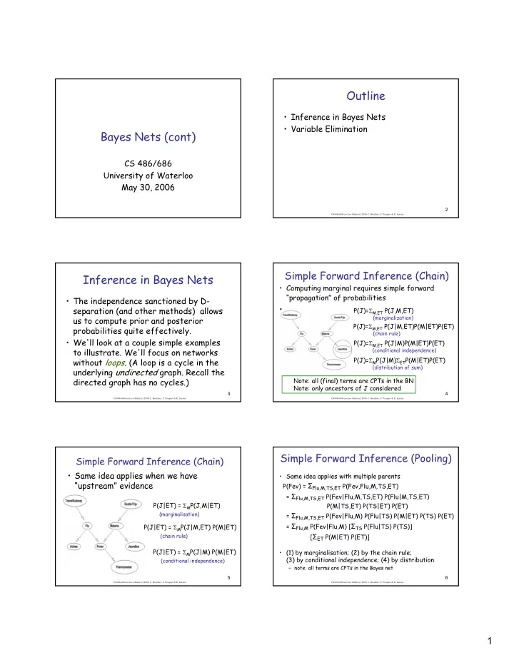
Outline • Inference in Bayes Nets • Variable Elimination Bayes Nets (cont) CS 486/686 University of Waterloo May 30, 2006 2 CS486/686 Lecture Slides (c) 2006 C. Boutilier, P. Poupart & K. Larson Simple Forward Inference (Chain) Inference in Bayes Nets • Computing marginal requires simple forward “propagation” of probabilities • The independence sanctioned by D- • separation (and other methods) allows P(J)= Σ M,ET P(J,M,ET) (marginalization) us to compute prior and posterior P(J)= Σ M,ET P(J|M,ET)P(M|ET)P(ET) probabilities quite effectively. (chain rule) • We'll look at a couple simple examples P(J)= Σ M,ET P(J|M)P(M|ET)P(ET) to illustrate. We'll focus on networks (conditional independence) P(J)= Σ M P(J|M) Σ ET P(M|ET)P(ET) without loops . (A loop is a cycle in the (distribution of sum) underlying undirected graph. Recall the directed graph has no cycles.) Note: all (final) terms are CPTs in the BN Note: only ancestors of J considered 3 4 CS486/686 Lecture Slides (c) 2006 C. Boutilier, P. Poupart & K. Larson CS486/686 Lecture Slides (c) 2006 C. Boutilier, P. Poupart & K. Larson Simple Forward Inference (Pooling) Simple Forward Inference (Chain) • Same idea applies when we have • Same idea applies with multiple parents “upstream” evidence P(Fev) = Σ Flu,M,TS,ET P(Fev,Flu,M,TS,ET) = Σ Flu,M,TS,ET P(Fev|Flu,M,TS,ET) P(Flu|M,TS,ET) P(J|ET) = Σ M P(J,M|ET) P(M|TS,ET) P(TS|ET) P(ET) (marginalisation) = Σ Flu,M,TS,ET P(Fev|Flu,M) P(Flu|TS) P(M|ET) P(TS) P(ET) = Σ Flu,M P(Fev|Flu,M) [ Σ TS P(Flu|TS) P(TS)] P(J|ET) = Σ M P(J|M,ET) P(M|ET) (chain rule) [ Σ ET P(M|ET) P(ET)] P(J|ET) = Σ M P(J|M) P(M|ET) • (1) by marginalisation; (2) by the chain rule; (3) by conditional independence; (4) by distribution (conditional independence) – note: all terms are CPTs in the Bayes net 5 6 CS486/686 Lecture Slides (c) 2006 C. Boutilier, P. Poupart & K. Larson CS486/686 Lecture Slides (c) 2006 C. Boutilier, P. Poupart & K. Larson 1
Simple Backward Inference Simple Forward Inference (Pooling) • Same idea applies with evidence • When evidence is downstream of query variable, we must reason “backwards.” This requires the P(Fev|ts,~m) = Σ Flu P(Fev,Flu|ts,~m) use of Bayes rule: P(ET | j) = α P(j | ET) P(ET) = Σ Flu P(Fev |Flu,ts,~m) P(Flu|ts,~m) = α Σ M P(j,M|ET) P(ET) = Σ Flu P(Fev|Flu,~m) P(Flu|ts) = α Σ M P(j|M,ET) P(M|ET) P(ET) = α Σ M P(j|M) P(M|ET) P(ET) • First step is just Bayes rule – normalizing constant α is 1/P(j); but we needn’t compute it explicitly if we compute P(ET | j) for each value of ET: we just add up terms P(j | ET) P(ET) for all values of ET (they sum to P(j)) 7 8 CS486/686 Lecture Slides (c) 2006 C. Boutilier, P. Poupart & K. Larson CS486/686 Lecture Slides (c) 2006 C. Boutilier, P. Poupart & K. Larson Backward Inference (Pooling) Variable Elimination • The intuitions in the above examples give us • Same ideas when several pieces of a simple inference algorithm for networks evidence lie “downstream” without loops: the polytree algorithm. P(ET|j,fev) = α P(j,fev|ET) P(ET) • Instead we'll look at a more general = α Σ M,Fl,TS P(j,fev,M,Fl,TS|ET) P(ET) algorithm that works for general BNs; but the polytree algorithm will be a special = α Σ M,Fl,TS P(j|fev,M,Fl,TS,ET) P(fev|M,Fl,TS,ET) P(M|Fl,TS,ET) P(Fl|TS,ET) P(TS|ET) P(ET) case. = α P(ET) Σ M P(j|M) Σ Fl P(fev|M,Fl) Σ TS P(Fl|TS) P(TS) • The algorithm, variable elimination , simply – Same steps as before; but now we compute prob of applies the summing out rule repeatedly. both pieces of evidence given hypothesis ET and – To keep computation simple, it exploits the combine them. Note: they are independent given M; independence in the network and the ability to but not given ET. distribute sums inward 9 10 CS486/686 Lecture Slides (c) 2006 C. Boutilier, P. Poupart & K. Larson CS486/686 Lecture Slides (c) 2006 C. Boutilier, P. Poupart & K. Larson Factors The Product of Two Factors • Let f( X , Y ) & g( Y , Z ) be two factors with • A function f(X 1 , X 2 ,…, X k ) is also called a variables Y in common factor . We can view this as a table of numbers, one for each instantiation of the • The product of f and g, denoted h = f x g variables X 1 , X 2 ,…, X k. (or sometimes just h = fg), is defined: – A tabular rep’n of a factor is exponential in k h( X , Y , Z ) = f( X , Y ) x g( Y , Z ) • Each CPT in a Bayes net is a factor: f(A,B) g(B,C) h(A,B,C) – e.g., Pr(C|A,B) is a function of three variables, ab 0.9 bc 0.7 abc 0.63 ab~c 0.27 A, B, C a~b 0.1 b~c 0.3 a~bc 0.08 a~b~c 0.02 • Notation: f( X , Y ) denotes a factor over the ~ab 0.4 ~bc 0.8 ~abc 0.28 ~ab~c 0.12 variables X ∪ Y . (Here X , Y are sets of ~a~b 0.6 ~b~c 0.2 ~a~bc 0.48 ~a~b~c 0.12 variables.) 11 12 CS486/686 Lecture Slides (c) 2006 C. Boutilier, P. Poupart & K. Larson CS486/686 Lecture Slides (c) 2006 C. Boutilier, P. Poupart & K. Larson 2
Restricting a Factor Summing a Variable Out of a Factor • Let f(X, Y ) be a factor with variable X ( Y • Let f(X, Y ) be a factor with variable X ( Y is a set) is a set) • We sum out variable X from f to produce • We restrict factor f to X=x by setting X to the value x and “deleting”. Define h = a new factor h = Σ X f, which is defined: f X=x as: h( Y ) = f(x, Y ) h( Y ) = Σ x ∊ Dom(X) f(x, Y ) f(A,B) h(B) = f A=a f(A,B) h(B) ab 0.9 b 0.9 ab 0.9 b 1.3 a~b 0.1 ~b 0.1 a~b 0.1 ~b 0.7 ~ab 0.4 ~ab 0.4 ~a~b 0.6 ~a~b 0.6 13 14 CS486/686 Lecture Slides (c) 2006 C. Boutilier, P. Poupart & K. Larson CS486/686 Lecture Slides (c) 2006 C. Boutilier, P. Poupart & K. Larson Variable Elimination: No Evidence Variable Elimination: No Evidence • Computing prior probability of query var X • Here’s the example with some numbers can be seen as applying these operations on factors A B C f 2 (A,B) f 3 (B,C) A B C f 1 (A) f 2 (A,B) f 3 (B,C) f 1 (A) f 1 (A) f 2 (A,B) f 3 (B,C) f 4 (B) f 5 (C) • P(C) = Σ A,B P(C|B) P(B|A) P(A) a 0.9 ab 0.9 bc 0.7 b 0.85 c 0.625 = Σ B P(C|B) Σ A P(B|A) P(A) ~a 0.1 a~b 0.1 b~c 0.3 ~b 0.15 ~c 0.375 = Σ B f 3 (B,C) Σ A f 2 (A,B) f 1 (A) ~ab 0.4 ~bc 0.2 = Σ B f 3 (B,C) f 4 (B) = f 5 (C) ~a~b 0.6 ~b~c 0.8 Define new factors: f 4 (B)= Σ A f 2 (A,B) f 1 (A) and f 5 (C)= Σ B f 3 (B,C) f 4 (B) 15 16 CS486/686 Lecture Slides (c) 2006 C. Boutilier, P. Poupart & K. Larson CS486/686 Lecture Slides (c) 2006 C. Boutilier, P. Poupart & K. Larson VE: No Evidence (Example 2) Variable Elimination: One View A • One way to think of variable elimination: f 1 (A) C D – write out desired computation using the chain f 4 (C,D) f 2 (B) B rule, exploiting the independence relations in f 3 (A,B,C) the network P(D) = Σ A,B,C P(D|C) P(C|B,A) P(B) P(A) – arrange the terms in a convenient fashion = Σ C P(D|C) Σ B P(B) Σ A P(C|B,A) P(A) – distribute each sum (over each variable) in as = Σ C f 4 (C,D) Σ B f 2 (B) Σ A f 3 (A,B,C) f 1 (A) far as it will go = Σ C f 4 (C,D) Σ B f 2 (B) f 5 (B,C) • i.e., the sum over variable X can be “pushed in” as far as the “first” factor mentioning X = Σ C f 4 (C,D) f 6 (C) – apply operations “inside out”, repeatedly = f 7 (D) eliminating and creating new factors (note Define new factors: f 5 (B,C), f 6 (C), f 7 (D), in the obvious that each step/removal of a sum eliminates way one variable) 17 18 CS486/686 Lecture Slides (c) 2006 C. Boutilier, P. Poupart & K. Larson CS486/686 Lecture Slides (c) 2006 C. Boutilier, P. Poupart & K. Larson 3
Recommend
More recommend
Explore More Topics
Stay informed with curated content and fresh updates.










![Bayesian Networks [KF] Chapter 3 University of Waterloo CS 786 Lecture 2: May 3rd, 2012](https://c.sambuz.com/996390/bayesian-networks-kf-chapter-3-s.webp)
