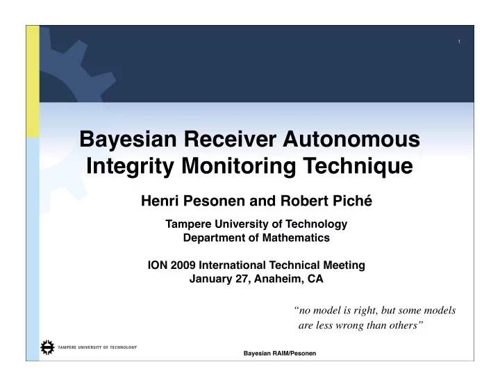
Bayesian Receiver Autonomous Integrity Monitoring Technique Henri - PowerPoint PPT Presentation

1 Bayesian Receiver Autonomous Integrity Monitoring Technique Henri Pesonen and Robert Piché Tampere University of Technology Department of Mathematics ION 2009 International Technical Meeting January 27, Anaheim, CA “no model is right, but some models are less wrong than others” Bayesian RAIM/Pesonen

Outline Motivation Traditional RAIM Bayesian model comparison Failure models Bayesian Receiver Autonomous Integrity Monitoring Method Simulations GPS-data test Conclusions Bayesian RAIM/Pesonen

Motivation Practically all GNSS-receivers implement RAIM in some form Detect & exclude faulty observations Decide of position estimate is reliable Almost all RAIM methods are based on statistical hypothesis tests Criticized for convoluted approach Alternative approach is Bayesian model comparison Bayesian RAIM/Pesonen

Traditional RAIM/FDE Classic RAIM/FDE is based on frequentist hypothesis testing Seek to reject hypothesis based on how unlikely it is RAIM/FDE as a two-stage procedure: global test local test H 0 H 1 , i H 0 , i α 0 α 0 2 2 H 1 T χ 2 1 − α , n − p Bayesian RAIM/Pesonen

Frequentist hypothesis testing Choose test statistic Choose significance level Find critical region Type I and II errors Assume we have correct models Test statistic realizes in critical region Two possible reasons: 1) H 0 wrong 2) sample is rare Assume sample is not rare ➔ H 0 is wrong “reject the null hypothesis with significance level α ” Bayesian RAIM/Pesonen

Bayesian model comparison Hypotheses (models) can be compared directly using Bayesian theory M P ( M i | D ) = P ( D | M i ) P ( M i ) Probability of a model given data P ( D ) “probability that the null hypothesis is true is P” Sometimes it is easier to think in terms of odds “What are the odds that the data is from one model?” Bayesian RAIM/Pesonen

Bayesian model comparison O i j = P ( M i | D ) � = P ( M i ) � × P ( D | M i ) The posterior odds � � � � M j | D D | M j M j P P P are the prior odds multiplied by the Bayes factor. Bayes factor is the ratio of evidences of models given the data Decisions can be made based on the odds O ij log 10 O ij Probability for M i against M j [1 , 3 . 2) [0 , 0 . 5) Not worth more than barely a mention [3 . 2 , 10) [0 . 5 , 1) Substantial [10 , 31 . 6) [1 , 1 . 5) Strong [31 . 6 , 100) [1 . 5 , 2) Very strong [100 , ∞ ) [2 , ∞ ) Decisive Bayesian RAIM/Pesonen

RAIM technique employing Bayesian model comparison theory Build statistical models for the observations (at most one failure at a time) M 0 : y = H 0 x 0 + v � x 0 � M i : y = H 0 x 0 + b i e i + v = [ H 0 , e i ] + v , i = 1 , . . ., n , b i � �� �� �� � H i ���� x i Prior distribution for the bias (in addition to state) Bayesian RAIM/Pesonen

Analytical formulation using normal distributions B i j = c i The Bayes factor × exp( g i ( z i ) − g j ( z j )) . c j   0 , i = 0 1 , i = 0  i ( z i ) = 1    g ∗  (( y − H i µ i ) T S − 1 e i ) 2   1 , i � 0 c ∗  , i � 0 i =  2 ×  i S − 1 e i + 1 e T �    σ 2  i S − 1 e i + 1 σ 2 b ( e T )  b  σ 2 b z i y − H i µ i g S = HP x 0 H T + R , = � P ( n − 1 channels are clean and 1 is contaminated) Prior P i 0 = P ( n channels are clean) P (channel is clean) n − 1 P (channel is contaminated) = P (channel is clean) n (1 − � ) n − 1 � � (16) = = (1 − � ) n 1 − � Bayesian RAIM/Pesonen

Position solution is the posterior distribution given the most plausible model Most probable model is the model with the best odds against the ‘null’ model k = arg max O i 0 i Position solution p ( x k | y, M k ) Use as a prior at next time step From posterior we can compute measures of quality How probable that the error is at most r ? Bayesian RAIM/Pesonen

Bayesian Receiver Autonomous Integrity Monitoring Method Condition for correct biased observation to be identified Best odds against the ‘null’ model Check if the odds for the best model are good enough Bayesian RAIM/Pesonen

Simulations We compare the detection performance of RAIM/FDE and BRAIM - :G98G R <# Observation noise +,*3"># C3 Every twenty epochs, one channel generates blunder 6 <# ,0# - :G9 ! 5 observations from Satellites generated uniformly on 9G< >#C3'#"$('77!('"#4')'#5'0')$('.#60 $057'#OY8G S 98G S PZOY8G S 98G S PZO8G S 98G S [8G R P# Tracks simulated using constant velocity model Bayesian RAIM/Pesonen

Simulations (large variance priors) < & & 8/1-& ! ; <=6)(0&>?& @AB & C1.2"2#& @AB & !1"7D.(& @AB & n 8GG R 9RGG R ? 8 9? R # S# CO! GL! J! H*%%$7)!9$7,&,*/! 8GG R 9RGG R # D 8 9D R # T# GG! CI! J! K%*/0!9$7,&,*/! 8GG R 9RGG R & U 8 9U R # V# ! $ % NJ 2 4& " MJ:C & E187(:$& E(6)& ! L & .(6D7)6& F")*& " MLJ 4& ! # @71.#(G51."123(&-."+.&/+.&-1.10()(.6B$& & Bayesian RAIM/Pesonen

Simulations (small variance priors) < & & <=6)(0&>?& @AB & C1.2"2#& @AB & !1"7D.(& @AB & 8/1-& ! ; n 8GG R 9RGG R I;! 3C! J! H*%%$7)!9$7,&,*/! ? 8 9? R # S# 8GG R 9RGG R # GG! CI! J! K%*/0!9$7,&,*/! D 8 9D R # T# & 8GG R 9RGG R & U 8 9U R # V# $ % NJ 2 4& " MJ:C & E187(9$& E(6)& ! L & .(6D7)6& F")*& " MLJ 4& ! # @60177G51."123(&-."+.&/+.&-1.10()(.6B$& ! Bayesian RAIM/Pesonen

GPS-data test BRAIM was tested using GPS-observations Artificial test was carried out by dropping good quality observations and by using the observation with the worst CNR 80 Kalman BRAIM 60 || error || 40 20 0 0 100 200 300 400 500 600 700 800 Epoch Bayesian RAIM/Pesonen

Summary Bayesian model comparison can be used as an alternative to traditional hypothesis test based-RAIM methods Frequentists: “reject the null hypothesis with significance level α ” Bayesians: “probability that the null hypothesis is true is P” BRAIM has Low computational complexity (under certain conditions) No restrictions on number of faulty observations (models) Natural expansion to time series Position domain investigations needed Bayesian RAIM/Pesonen

Thank you! Questions? www.math.tut.fi/posgroup henri.pesonen@tut.fi Bayesian RAIM/Pesonen