Outline Motivation - The Modia project Introduction to Modia - PDF document

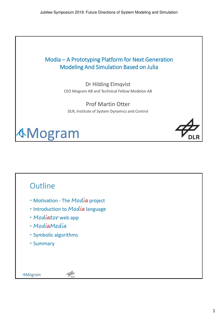
Jubilee Symposium 2019: Future Directions of System Modeling and Simulation Mo Modi dia – A A Prot ototyping Platform for or Ne Next Gene Generatio ion Mo Modelin ing And And Simula Simulatio ion Base Based d on on Jul Julia Dr Hilding Elmqvist CEO Mogram AB and Technical Fellow Modelon AB Prof Martin Otter DLR, Institute of System Dynamics and Control Outline  Motivation - The Modia project  Introduction to Modia language  Modiator web app  ModiaMedia  Symbolic algorithms  Summary 1

Jubilee Symposium 2019: Future Directions of System Modeling and Simulation Modelica Challenges  Modelica is powerful (equations, objects, connections)  Although static, requiring recompilation if:  An array dimension is changing  A component class is changing  A medium is changing  Modelica algorithms and functions lack functionalities:  Modern data structures  Parallelization  …  It is possible to build complex system models, but:  Sometimes hard to understand models (3D, media/fluid models, …)  Translation should be faster  Simulation should be faster Innovation platform - Modia Open source project consisting of several Based on modern language – Julia Julia packages (github.com/ModiaSim) Modia • Dynamic typing, Matlab-like notation Equation-based modeling • Static typing, efficient, data structures (as C++) Modiator 2D/3D model editor • Multiple dispatch ModiaMath • Metaprogramming Simulation environment • for domain specific language extensions Modia3D 3D geometry and 3D mechanics • for symbolic processing ModiaMedia • Thermodynamic property models Just-in-time compilation Modelia Modelica model importer (partial) Contributors : Hilding Elmqvist, Toivo Henningsson, Martin Otter, Andrea Neumayr, Oskar Åström, Chris Laughman 2

Jubilee Symposium 2019: Future Directions of System Modeling and Simulation Connectors and Components - Electrical Modelica @ model Pin begin connector Pin v=Float() Modelica.SIunits.Voltage v; i=Float(flow=true) flow Modelica.SIunits.Current I; end end Pin; @ model OnePort begin partial model OnePort p=Pin() SI.Voltage v; n=Pin() SI.Current i; v=Float() PositivePin p; i=Float() NegativePin n; @ equations begin equation v = p.v - n.v # Voltage drop v = p.v - n.v; 0 = p.i + n.i # KCL within component 0 = p.i + n.i; i = p.i i = p.i; end end OnePort; end model Resistor @ model Resistor begin # Ideal linear electrical resistor parameter Modelica.SIunits.Resistance R; @ extends OnePort() extends Modelica.Electrical.Analog.Interfaces.OnePort; @ inherits i, v equation R=1 # Resistance v = R*i; @ equations begin end Resistor; R*i = v end end Elmqvist/Henningsson/Otter 2017: Innovations for Future Modelica Coupled Models - Electrical Circuit Modelica model LPfilter @ model LPfilter begin Resistor R(R=100); R = Resistor(R=100) Capacitor C(C=0.001); C = Capacitor(C=0.001) ConstantVoltage V(V=10); V = ConstantVoltage(V=10) Ground ground; @ equations begin equation connect(R.n, C.p) connect(R.n, C.p); connect(R.p, V.p) connect(R.p, V.p); connect(V.n, C.n) connect(V.n, C.n); end connect(V.n, ground.p); end end Lpfilter; R R=100 ground 3

Jubilee Symposium 2019: Future Directions of System Modeling and Simulation Modiator – web app  Summer 2019 prototype  Summer intern: Oskar Åström  Joint project between Modelon and Mogram  Cooperation with Martin Otter, DLR  Modelica diagrams  Exploring fundamentals  CSG – Constructive Solid Modeling  Shape parametrization  Focus: 3D model composition and animation  Modia3D  Modelica … MultiBody 3D model composition • Mechanism composition • Introducing joints • Parametrization • Immediate kinematic animation • Exploded view 4

Jubilee Symposium 2019: Future Directions of System Modeling and Simulation 3D Animation Generate Modia3D model •  Determine properties from geometries (mass, ...)  3D mechanics algorithms  Collision handling  Fast translation • Client/server communication between web app and Julia • Simulate Animate result in Modiator • Modelica Multibody 3D parametric preview • Kinematic animation • Parametric animation • Spanning tree view • Interpretation of Modelica AST • Evaluation of Modelica expressions 5

Jubilee Symposium 2019: Future Directions of System Modeling and Simulation ModiaMedia - Thermodynamic property models Developers: Martin Otter (DLR), Hilding Elmqvist (Mogram), Chris Laughman (MERL); Paper at Modelica‘2019 using ModiaMedia Medium = getMedium("N2") # dictionary p = 1e5 T = 300.0 state = setState_pT(Medium, p, T) # construct setState_pT!(state, 2*p, 2*T) # update d = density( state ) # get other properties h = specificEnthalpy( state ) listMedia() # list all supported media standardPlot(Medium) # plot Medium • Much simpler and more powerful as Modelica.Media • Fluid network: state propagated/updated along connection structure (Medium defined at one state instance) Symboli lic Algorit ithms For 𝟏 = 𝐠 𝐲 , 𝐲, 𝑢 • • Can be used directly in current Modelica tools 6

Jubilee Symposium 2019: Future Directions of System Modeling and Simulation Modelica translation today - flattening  Object-oriented modeling approach  allows building large models with millions of equations  Semantic specification is based on flattening  i.e. cloning variables and equations of each component instance  And most tools also expands matrix equations Negative consequences:  A lot of memory is needed for variables and equations during translation  Translation time is unnecessary long  same analysis (flattening, symbolic processing, etc) is performed repeatedly for each instance of a component  C-code gets large and compilation takes long time 16 Remedy: Separate Translation  Parts of the equations of a component  are always executed in the same order and with the same causality  independently of how the component is connected  Such sequences of equations can be put into functions  which are reused for all components of the same class  less C-code gives shorter compilation time  Finding such sequences can be made once for each model class  faster translation and less memory use 17 7

Jubilee Symposium 2019: Future Directions of System Modeling and Simulation Component Model Equations DAE: 𝑔(𝑦 , 𝑦, 𝑑 𝑞 , 𝑑 𝑔 , 𝑣, 𝑧, 𝑤, 𝑞) =0  𝑦 – differentiated variables  𝑑 𝑞 – potentials of the connectors  𝑑 𝑔 – flows and streams of the connectors  u – inputs  y – outputs  v – other variables  p – parameters  dim( 𝑔 ) = dim( 𝑦 )+dim( 𝑑 𝑞 )+dim( 𝑧 )+dim( 𝑤 ) Generic environment of model:  Generic environment needs to relate all connector variables  𝑕(𝑑 𝑞 , 𝑑 𝑔 , 𝑣, 𝑧) =0  dim( 𝑕 ) = dim( 𝑑 𝑔 )+dim( 𝑣 )  𝑕 has full incidence  Might also contain derivatives Model equations partitioning Perform BLT on f and g function incidences  First blocks (always same causality, use function): 𝑑 𝑞 , 𝑑 𝑔 , 𝑣  𝑦 1 , 𝑧 1 , 𝑤 1 = 𝑔 1 (𝒚, 𝒒) f 1  Middle block ( 𝑔 2 kept as equations): g, f 2  𝑕(𝑑 𝑞 , 𝑑 𝑔 , 𝑣, 𝑧) =0 f 3  𝑔 2 (𝒚 𝟐 , 𝑦 2 , 𝒚, 𝑑 𝑞 , 𝑑 𝑔 , 𝑣, 𝒛 𝟐 , 𝑧 2 , 𝒘 𝟐 , 𝑤 2 , 𝒒) =0 Since g has full incidence, all g-equations  Last blocks (always same causality, use function): will appear in the same block  𝑦 3 , 𝑧 3 , 𝑤 3 = 𝑔 3 (𝒚 𝟐 , 𝒚 𝟑 , 𝒚, 𝒅 𝒒 , 𝒅 𝒈 , 𝒗, 𝒛 𝟐 , 𝒛 𝟑 , 𝒘 𝟐 , 𝒘 𝟑 , 𝒒) Known variables marked in bold face 8

Jubilee Symposium 2019: Future Directions of System Modeling and Simulation name Example: Heat exchanger model MSL BasicHX  flow models close to connectors  10 spatial segments f1  50 dynamic states f2  514 equations g  dim(f2) = 24 f3 axis6 Example: Multibody Robot model a b axis5 n={1,0,0} r5 axis4 MSL Robot with der(phi) r3 n={1,0,0} b a axis3  With der(phi) in g(…) a b axis2 n={1,0,0} r2 f1 to enable connecting dampers axis1 y world  12 dynamic states x g  391 equations  dim(f2) = 0 f3  Modia3D is a manual implementation of this approach 9