Semantic Guidance (and other methods) for Saturation Provers 8th - PowerPoint PPT Presentation
Semantic Guidance (and other methods) for Saturation Provers 8th International Conference on ARTIFICIAL INTELLIGENCE AND SYMBOLIC COMPUTATION Beihang University, Beijing, September 2006 William McCune Downers Grove, Illinois U.S.A. An
Semantic Guidance (and other methods) for Saturation Provers 8th International Conference on ARTIFICIAL INTELLIGENCE AND SYMBOLIC COMPUTATION Beihang University, Beijing, September 2006 William McCune Downers Grove, Illinois U.S.A.
An Equational Problem f ( f ( y, x ) , f ( f ( f ( x, x ) , z ) , f ( f ( f ( f ( f ( x, y ) , z ) , z ) , x ) , f ( x, u )))) = x ? ⇒ f ( x, f ( y, f ( x, f ( z, z )))) = f ( x, f ( z, f ( x, f ( y, y )))) 2
Saturation Provers for First-order and Equational Logic • Inference – Proof by refutation – Make inferences (under some restrictions), keeping formulas simplified • Completeness – If the conjecture is a theorem, a proof will eventually be found • Strategy – Term ordering for inference and simplification – Selection function for application of inference rules – Special-purpose strategies (may be incomplete) • Examples: Otter, E, Vampire, Waldmeister, Prover9 3
The Inference Loop • Maintain two sets of formulas – active : available for making inferences – passive : waiting to participate in the search • Loop: – Select a formula C from passive (the given clause ); – move C from passive to active ; – make inferences from C and other formulas in active ; – simplify inferred formulas and append to passive ; • Two versions: Otter loop and Discount loop – differ on when and how simplification occurs 4
Theory vs. Practice Completeness Results • Even though an inference is not needed, – it might be very helpful in practice. • Even though an inference may be necessary in general, – it might be wasteful in practice. Restriction vs. Guidance • Restriction: Constrain application of inference rules • Guidance: Selection of the given clause 5
Three Promising Strategies 1. Semantic Guidance – using interpretations to help select the given clause 2. Variable Ordering – extending the term ordering with variables – ( y ∗ x ) ≻ ( x ∗ y ) – incomplete 3. Introduce Equational Definitions – emphasize “important” terms, e.g., g ( x, y ) = f ( f ( x, x ) , f ( y, y )) 6
Programs for Experimenting with Strategies • Prover9 – theorem prover for first-order and equational logic – Otter’s (and EQP’s) successor • Mace4 – searches for finite models and counterexamples 7
Semantic Guidance Using interpretations to help select the given clause 8
Semantic Inference Rules for First-order and Equational Deduction • Based on interpretations (explicit or implicit, finite or infinite) • Semantic Resolution (Slagle 1965) – given an interpretation I , for each (binary) inference, at least one parent must be false in I . – example: positive resolution uses the (implicit) interpretation in which all atomic formulas are false. • Set of support resolution (Wos, 1964): justified by any interpretation of the axioms, and the semantic restriction applies only to input clauses. 9
Semantic Inference Rules (continued) • Semantic Paramodulation • Semantic Resolution for Horn Sets (Henschen 1976) – If one of the parents is a positive unit false in I , the child must also be false in I . – applies also to paramodulation 10
Semantic Inference with Explicit Interpretations • not much work, not much success – incompatibilities with inference rules based on term orderings and simplifi- cation • Powerful finite-model finding programs, starting about 1990 – Finder, MGTP , Mace2, Falcon, SEM, Mace4, Paradox. • The SCOTT series of provers (Slaney, Hodgson, et al). – dynamic interpretations, partial interpretations, multiple interpretations – guidance and well as restriction 11
Semantic Guidance • Assume the Otter loop or the Discount loop . • Selecting the next clause for making inferences (the given clause ). – weighting function: lightest first – age: breadth first – age/weight ratio • For semantic guidance, specify a 3-way ratio: – age, – lightest clause false in I , – lightest clause true in I . 12
Lattice Theory Example: The Problem In lattice theory (LT), what is the relationship between the following two identi- ties? x ∧ ( y ∨ ( x ∧ z )) = x ∧ ( y ∨ ( z ∧ (( x ∧ ( y ∨ z )) ∨ ( y ∧ z )))) (H2) ( x ∧ y ) ∨ ( x ∧ z ) = x ∧ (( y ∧ ( x ∨ z )) ∨ ( z ∧ ( x ∨ y ))) (H82) • LT, H2 → H82 ? No . Mace4 easily finds a counterexample of size 6. • LT, H82 → H2 ? Semantic guidance for LT, H82 → H2 • The conjecture has the form theory, hypotheses → conclusion . • Consider a lattice (the theory) in which the H2 (the conclusion) is false. 13
Lattice Theory Example: Guiding Interpretation Mace4 Input formulas(assumptions). % Lattice theory x v y = y v x. (x v y) v z = x v (y v z). x ˆ y = y ˆ x. (x ˆ y) ˆ z = xˆ (y ˆ z). x ˆ (x v y) = x. x v (x ˆ y) = x. end_of_list. formulas(goals). % falsify these formulas x ˆ (y v (x ˆ z)) = x ˆ (y v (z ˆ ((x ˆ (y v z)) v (y ˆ z)))) # label(H2). end_of_list. 14
Lattice Theory: Guiding Interpretation Mace4 Result interpretation( 6, [number=1, seconds=0], [ function(c1, [2]), function(c2, [3]), function(c3, [4]), function(ˆ(_,_), [ 0, 0, 0, 0, 0, 0, 0, 1, 2, 3, 4, 5, 0, 2, 2, 0, 0, 0, 0, 3, 0, 3, 5, 5, 0, 4, 0, 5, 4, 5, 0, 5, 0, 5, 5, 5]), function(v(_,_), [ 0, 1, 2, 3, 4, 5, 1, 1, 1, 1, 1, 1, 2, 1, 2, 1, 1, 1, 3, 1, 1, 3, 1, 3, 4, 1, 1, 1, 4, 4, 5, 1, 1, 3, 4, 5])]). 15
Lattice Theory: Search with Guiding Interpretation • Give Prover9 the guiding interpretation. • Tell Prover9 to use the selection ratio (age=1 : false=4 : true=1). • Proof in 10 seconds. • Proof in 1 hour without guidance. How does the interpretation help to find a proof? 16
A Chain of Varieties: LT, OL, OML, MOL, BA As structures (algebras): Lattices (LT) Ortholattices (OL) Orthomodular Lattices (OML) Modular Ortholattices (MOL) Boolean Algebras (BA) 17
A Chain of Varieties: LT, OL, OML, MOL, BA Lattice Theory (LT) ( x ∨ y ) ∨ z = x ∨ ( y ∨ z ) . ( x ∧ y ) ∧ z = x ∧ ( y ∧ z ) . x ∨ y = y ∨ x. x ∧ y = y ∧ x. x ∨ ( x ∧ y ) = x. x ∧ ( x ∨ y ) = x. For Ortholattices (OL), include a unary operation with the following constraints. x ∧ y = ( x ′ ∨ y ′ ) ′ . x ′′ = x. x ∨ x ′ = 1 . For Orthomodular Lattices (OML), add the following constraint. x ∨ ( x ′ ∧ ( x ∨ y )) = x ∨ y. For Modular Ortholattices (MOL), add the following constraint. x ∨ ( y ∧ ( x ∨ z )) = x ∨ ( z ∧ ( x ∨ y )) . For Boolean Algebras (BA), add the following constraint. x ∨ ( y ∧ z ) = ( x ∨ y ) ∧ ( x ∨ z ) . 18
Modular Ortholattice (MOL) Single Axiom: The Problems Consider the equations f ( f ( y, x ) , f ( f ( f ( x, x ) , z ) , f ( f ( f ( f ( f ( x, y ) , z ) , z ) , x ) , f ( x, u )))) = x (MOL) f ( x, f ( y, f ( x, f ( z, z )))) = f ( x, f ( z, f ( x, f ( y, y )))) (M) f ( x, f ( f ( y, z ) , f ( y, z ))) = f ( y, f ( f ( x, z ) , f ( x, z ))) (A) • (MOL) is a single axiom for modular ortholattices in terms of the Sheffer stroke (NAND). • Problem 1 (modularity property): (MOL) → (M). • Problem 2 (associativity property): (MOL) → (A). 19
MOL Single Axiom: Selecting Interpretations • Modularity property. – Consider the chain of varieties: OL, OML, MOL, BA (Ortholattices, Orthomodular Lattices, Modular Ortholattices, Boolean Algebra). – Let OML be the “theory”, and use the smallest non-modular OML (size 10) to guide the search. – Proof in 10 minutes with guidance; proof in 50 minutes without. • Associativity property. – How do we find a nonassociative “theory” in which to work? – Simple answer: Consider nonassociative interpretations that satisfy other MOL properties. Pick one of size 8. – Proof in 44 seconds with guidance; proof in 162 seconds without. 20
Variable Ordering Extending the term ordering with variables 21
Variable Ordering: Background • Proof search based on term ordering and term rewriting. • A simplification ordering allows equations to be used as rewrite rules. – E.g., KBO (Knuth-Bendix Ordering), LPO (Lexicographic Path Ordering). • Ordinarily, term rewriting always produces smaller terms. – Orientable rules, e.g, x ′′ = x , are always applied. – A non-orientable rule, e.g., x ∗ y = y ∗ x , is applied only if it produces a smaller term. • Many proof procedures based on these term orderings are complete . 22
Variable Ordering: An Incomplete Strategy • When deciding whether to apply a non-orientable rewrite rule, include vari- ables in the term ordering: variables ≺ constants x ≺ y ≺ z ≺ u ≺ v ≺ · · · In other words, treat variables as constants when comparing terms. • We have no theoretical basis for this method. • The method is incomplete (it can block all proofs). • It can be used with KBO or with LPO. 23
Variable Ordering: Median Algebra Problem Axioms for Median Algebra f ( x, y, z ) = f ( z, x, y ) f ( x, y, z ) = f ( x, z, y ) f ( x, x, y ) = x f ( f ( x, w, y ) , w, z ) = f ( x, w, f ( y, w, z )) Conclusion f ( f ( x, y, z ) , u, w ) = f ( x, f ( y, u, w ) , f ( z, u, w )) • Note that the first two axioms allow the arguments to be permuted in any way. 24
Recommend
More recommend
Explore More Topics
Stay informed with curated content and fresh updates.
