Outline Introduction (9.1) Analysis of Paired Samples (9.2) - PDF document

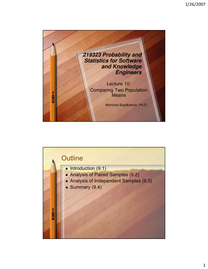
1/26/2007 219323 Probability and Statistics for Software Statistics for Software and Knowledge Engineers Lecture 10: Comparing Two Population Comparing Two Population Means Monchai Sopitkamon, Ph.D. Outline � Introduction (9.1) � Analysis of Paired Samples (9.2) � Analysis of Independent Samples (9.3) � Summary (9.4) 1

1/26/2007 Comparing Two Population Means: Introduction I (9.1) � Two-Sample Problems – making comparisons between two prob distributions comparisons between two prob distributions � Comparing two distributions by comparing their means and probably variances � If the means are equal, may be enough to conclude that the populations are “identical” Comparing Two Population Means: Introduction II (9.1) Comparison of the means Comparison of the of two variances of two probability distributions probability distributions 2

1/26/2007 Comparing Two Population Means: Introduction III (9.1) μ A = μ B ? Kudzu pulping experiment Comparing Two Population Means: Introduction IV (9.1) Interpretation of confidence intervals for µ A − µ B 3

1/26/2007 Comparing Two Population Means: Introduction V (9.1) � A more direct approach to assessing the plausibility that the population means μ A and plausibility that the population means μ A and μ B are equal is to calculate a p -value for the hypotheses H 0 : μ A = μ B versus H A : μ A ≠ μ B if p -value < 0.01 � accept H A if p -value > 0.1 � accept H 0 Paired Samples Versus Independent Samples I (9.1.2) � Experimental design methodology p provides different ways of collecting and y g analyzing data for comparison of two populations. � Ex.55 pg.386: Heart Rate Reductions A new drug for inducing temporary patient’s heart rate reduction is to be compared with a standard drug. 40 patients are given at random a new drug on 40 patients are given, at random, a new drug on day 1 and a standard drug on day 2, and vice versa. Comparison based on the differences for each patient in the percentage heart rate reductions achieved by the two drugs. 4

1/26/2007 Paired Samples Versus Independent Samples II (9.1.2) Heart rate reduction experiment Paired Samples Versus Independent Samples III (9.1.2) “Blocking” Equal sample size The distinction between paired and independent samples 5

1/26/2007 Paired Samples Versus Independent Samples IV (9.1.2) Variability in patients creates more “noisy” d data, which may not hi h yield accurate interpretation of results! Therefore, paired experiment is more efficient ! efficient ! Unpaired design for heart rate reduction experiment Outline � Introduction (9.1) � Analysis of Paired Samples (9.2) � Analysis of Independent Samples (9.3) � Summary (9.4) 6

1/26/2007 Analysis of Paired Samples I (9.2) � Paired samples w/ data observations ( x ( x 1 , y 1 ), ( x 2 , y 2 ), …, ( x n , y n ) y ) ( x y ) ( x y ) is performed by reducing problem to one- sample problem, by calculating z i = x i – y i 1 ≤ i ≤ n z i � independent, identically distributed observations from some prob dist w/ mean observations from some prob dist w/ mean μ . μ � average difference between “treatments” A and B Analysis of Paired Samples II (9.2) � If μ > 0 � RVs X i tends to be > RVs Y i , or μ A > μ B μ B � If μ < 0 � RVs X i tends to be < RVs Y i , or μ A < μ B � Perform two-sided hypotheses test H 0 : μ = 0 versus H A : μ ≠ 0 and compute p -value and evaluate it p p accordingly. 7

1/26/2007 Analysis of Paired Samples III (9.2) � Ex.55 pg.390: Heart Rate Reductions t = -4.50 Two-sided hypothesis test H 0 : μ = 0 versus H A : μ ≠ 0 w/ the computed p -value = 0.00006 ≅ 0.001 � reject null hypothesis H 0 which means new drug has a g different effect from the standard drug Heart rate reductions data set (% reduction in heart rate) Excel sheet Two-Sided Hypothesis Test for a Population Mean ( ) − μ n x = 0 t s Size α two- sided t -test 8

1/26/2007 Outline � Introduction (9.1) � Analysis of Paired Samples (9.2) � Analysis of Independent Samples (9.3) � Summary (9.4) Analysis of Independent Samples I (9.3) � Two independent (unpaired) samples � Three procedures can be applied depending on depending on 1. the sample size (if large � proc 1), Two-sample 2. if sample size is small and if the population t -tests variances are equal (proc 2), 3. if the population variances are known (proc Two-sample 3) z -test 9

1/26/2007 Analysis of Independent Samples: General Procedure I (9.3.1) Two-Sample t -Procedure (Unequal Variances) A two-sided 1 - α level CI for the difference in population means μ A - μ B is ⎛ ⎞ 2 2 2 2 ⎜ s s ⎟ s s μ − μ ∈ − − + − + + y y x x x y t , x y t ⎜ ⎟ α ν α ν A B / 2 , / 2 , n m n m ⎝ ⎠ where the degrees of freedom of critical point is 2 ⎛ ⎞ 2 2 + s s ⎜ ⎟ + y x ⎜ ⎜ ⎟ ⎟ ⎝ n m ⎠ ν = 4 4 s s + y x − − 2 2 ( 1 ) ( 1 ) n n m m One-sided CIs are ⎛ ⎞ ⎛ ⎞ 2 2 2 s 2 s ⎜ s ⎟ ⎜ s ⎟ and μ − μ ∈ − ∞ − + + μ − μ ∈ − − + ∞ y y x , x y t x x y t , ⎜ ⎟ ⎜ ⎟ α ν α ν A B , A B , n m n m ⎝ ⎠ ⎝ ⎠ Analysis of Independent Samples: General Procedure II (9.3.1) � The appropriate t -statistic for the null hypothesis H 0 : μ A - μ B = δ is 0 μ A μ B yp − − δ x y = t 2 2 s s + y x n m � Two-sided p -value = 2x P ( X > | t |), where X has t- distribution w/ ν degrees of freedom � One sided p value = P ( X > t ) and P ( X < t ) � One-sided p -value = P ( X > t ) and P ( X < t ) � A size α two-sided hypothesis test accepts H 0 if | t | ≤ t α /2, ν and rejects H 0 if | t | > t α /2, ν � Size α one-sided hypothesis tests have rejection regions t > t α , ν or t < - t α , ν 10

1/26/2007 Analysis of Independent Samples: General Procedure III (9.3.1) 24 34 n m x y 9.005 11.864 s s 3.438 3.305 y x The hypotheses H 0 : μ A = μ B versus H A : μ A ≠ μ B are tested w/ t -statistic − − δ − − x y 9 . 005 11 . 864 0 = = = − t 3 . 169 2 2 2 2 s 3 . 438 3 . 305 s + + y x 24 34 n m Excel sheet Analysis of Independent Samples: General Procedure IV (9.3.1) � Two-sided p -value = 2x P ( X >|-3.169|) = 2x 2x P ( X >3.169) 2x P ( X 3.169) where X has t -distribution w/ dof. 2 ⎛ ⎞ 2 2 ⎛ ⎞ 2 s s 2 2 ⎜ ⎟ 3 . 348 3 . 305 + ⎜ + ⎟ y x ⎜ ⎟ ⎜ ⎟ ⎝ n m ⎠ ⎝ ⎠ 24 34 ν = = = ≅ 48 . 43 48 4 4 4 4 3 . 348 3 . 305 s s + + y x × × − − 2 2 2 2 24 23 34 33 n ( n 1 ) m ( m 1 ) p -value ≅ 2x0 00135 = 0 0027 p -value ≅ 2x0.00135 = 0.0027 since 0.0027 < 0.01 � null hypothesis H 0 : μ A = μ B is rejected, and it can be concluded that μ A ≠ μ B Excel sheet 11

1/26/2007 Analysis of Independent Samples: General Procedure V (9.3.1) Calculation of a two-sided p -value Analysis of Independent Samples: General Procedure VI (9.3.1) � Construct a two-sided 99% CI for the difference in population means μ A – μ B , using critical point t α /2 ν = t 0 005 48 = 2.6822 α /2, ν 0.005,48 ⎛ ⎞ 2 2 2 2 ⎜ s s ⎟ s s μ − μ ∈ − − + − + + y y x x x y t , x y t ⎜ ⎟ α ν α ν A B / 2 , / 2 , n m n m ⎝ ⎠ ⎛ ⎞ 2 2 3 . 438 3 . 305 ⎜ ⎟ − − + 9 . 005 11 . 864 2 . 6822 , ⎜ ⎟ 24 34 = ⎜ ⎟ ⎜ 2 2 ⎟ 3 . 438 3 . 305 − + + + + ⎜ ⎜ ⎟ ⎟ 9 9 . 005 005 11 11 . 864 864 2 2 . 6822 6822 ⎝ ⎠ 24 34 ( ) = − − 5 . 28 , 0 . 44 CI does not include 0 implies that H 0 : μ A = μ B has a two-sided p -value < 0.01, consistent w/ the result of the hypothesis test shown in the previous slides Excel sheet 12

1/26/2007 Analysis of Independent Samples: General Procedure VII (9.3.1) Relationship between hypothesis testing R l ti hi b t h th i t ti and confidence intervals for two-sample two-sided problems Analysis of Independent Samples: Pooled Variance Procedure I (9.3.2) � For small sample sizes and when population variances are equal ( ( ) ) variances are equal σ = σ = σ 2 2 2 A A B B ( ) ( ) − + − 2 2 Pooled variance 1 1 n s m s σ = = x y 2 2 ˆ s + − p estimator: n m 2 � Consider the previous example. Since the sample SDs are similar, it could be assumed that the population variances are equal. p p q Therefore, the estimated common SD is ( ) ( ) − + − × + × 2 2 2 2 n 1 s m 1 s ( 23 3 . 438 ) ( 33 3 . 305 = = x y s + − + − p n m 2 24 34 2 = 3 . 360 Excel sheet 13

1/26/2007 Analysis of Independent Samples: Pooled Variance Procedure II (9.3.2) � The hypotheses H : μ = μ H 0 : μ A = μ B H : μ ≠ μ H A : μ A ≠ μ B versus versus are tested w/ t -statistic − − 9 . 005 11 . 864 x y = = = − t 3 . 192 1 1 1 1 + + s 3 . 360 p n m 24 34 The two-sided p -value = 2x P ( X > |-3.192|) = 2x P ( X > 3.192) ≅ 2x0.00115 = 0.0023 where X has t -distribution w/ dof n + m -2 = 56 as shown in the next figure. Excel sheet Analysis of Independent Samples: Pooled Variance Procedure III (9.3.2) Calculation of a two-sided p -value 14