Radial basis function partition of unity methods for PDEs RBF-PUM - - PowerPoint PPT Presentation

RBF-PUM

Outline Introduction RBF–PUM Theoretical results Numerical results RBF-QR Convergence Robustness 3-D results Cost Adaptivity Summary

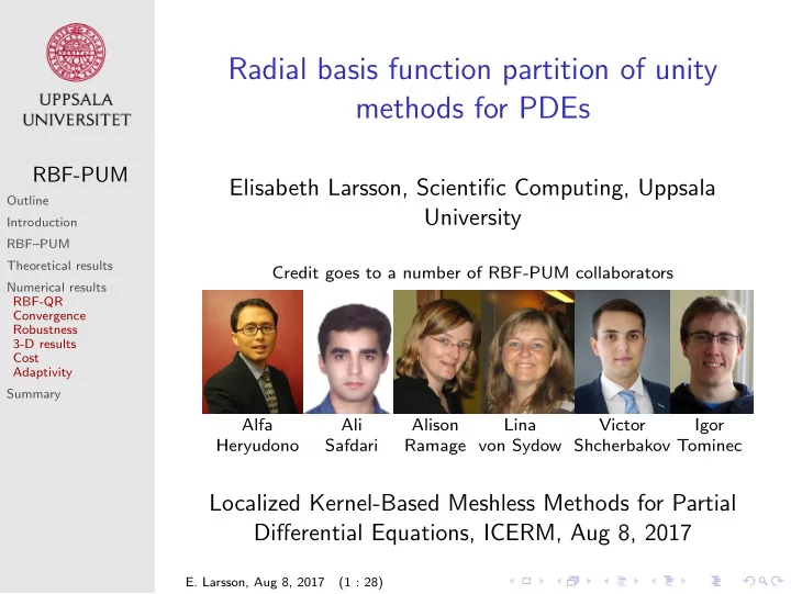
Radial basis function partition of unity methods for PDEs

Elisabeth Larsson, Scientific Computing, Uppsala University

Credit goes to a number of RBF-PUM collaborators Alfa Ali Alison Lina Victor Igor Heryudono Safdari Ramage von Sydow Shcherbakov Tominec

Localized Kernel-Based Meshless Methods for Partial Differential Equations, ICERM, Aug 8, 2017

• E. Larsson, Aug 8, 2017

(1 : 28)

RBF-PUM

Outline Introduction RBF–PUM Theoretical results Numerical results RBF-QR Convergence Robustness 3-D results Cost Adaptivity Summary

Outline

Introduction RBF partition of unity methods for PDEs Theoretical results Numerical results RBF-QR Convergence Robustness 3-D results Cost Adaptivity Summary

• E. Larsson, Aug 8, 2017

(2 : 28)

RBF-PUM

Outline Introduction RBF–PUM Theoretical results Numerical results RBF-QR Convergence Robustness 3-D results Cost Adaptivity Summary

Motivation for RBF-PUM

Global RBF approximation

+ Ease of implementation in any dimension. + Flexibility with respect to geometry. + Potentially spectral convergence rates. − Computationally expensive for large problems.

RBF-PUM

◮ Local RBF approximations on patches are blended

into a global solution using a partition of unity.

◮ Provides spectral or high-order convergence. ◮ Solves the computational cost issues. ◮ Allows for local adaptivity.

Wendland (2002), Fasshauer (2007), Cavoretto, De Rossi, Perracchione et al., Larsson, Heryudono et al.

• E. Larsson, Aug 8, 2017

(3 : 28)

RBF-PUM

Outline Introduction RBF–PUM Theoretical results Numerical results RBF-QR Convergence Robustness 3-D results Cost Adaptivity Summary

The RBF partition of unity method

Ωj

Global approximation

˜ u(x) =

P

• j=1

wj(x)˜ uj(x)

PU weight functions

Generate weight functions from compactly supported C 2 Wendland functions ψ(ρ) = (4ρ + 1)(1 − ρ)4

+

using Shepard’s method wi(x) =

ψi(x) M

j=1 ψj(x).

Cover

Each x ∈ Ω must be in the interior of at least one Ωj. Patches that do not contain unique points are pruned.

• E. Larsson, Aug 8, 2017

(4 : 28)

RBF-PUM

Outline Introduction RBF–PUM Theoretical results Numerical results RBF-QR Convergence Robustness 3-D results Cost Adaptivity Summary

Differentiating RBF-PUM approximations

100 200 300 50 100 150 200 250 300 350 nz = 10801

Applying an operator globally

∆˜ u =

M

• i=1

∆wi ˜ ui + 2∇wi · ∇˜ ui + wi∆˜ ui

Local differentiation matrices

Let ui be the vector of nodal values in patch Ωi, then ui = Aλi, where Aij = φj(xi) ⇒ Lui = ALA−1ui, where AL

ij = Lφj(xi).

The global differentiation matrix

Local contributions are added into the global matrix.

• E. Larsson, Aug 8, 2017

(5 : 28)

RBF-PUM

Outline Introduction RBF–PUM Theoretical results Numerical results RBF-QR Convergence Robustness 3-D results Cost Adaptivity Summary

An RBF-PUM collocation method

Choices & Implications

◮ Nodes and evaluation points coincide.

Square matrix, iterative solver available (Heryudono, Larsson, Ramage, von Sydow 2015).

◮ Global node set.

Solutions ˜ ui(xk) = ˜ uj(xk) for xk in overlap regions.

◮ Patches are cut by the domain boundary.

Potentially strange shapes and lowered local order.

• E. Larsson, Aug 8, 2017

(6 : 28)

RBF-PUM

Outline Introduction RBF–PUM Theoretical results Numerical results RBF-QR Convergence Robustness 3-D results Cost Adaptivity Summary

An RBF-PUM least squares method

Choices & Implications

◮ Each patch has an identical node layout.

Computational cost for setup is drastically reduced.

◮ Evaluation nodes are uniform.

Easy to generate both local and global high quality node sets.

◮ Patches have nodes outside the domain.

Good for local order, but requires denser evaluation points.

• E. Larsson, Aug 8, 2017

(7 : 28)

RBF-PUM

Outline Introduction RBF–PUM Theoretical results Numerical results RBF-QR Convergence Robustness 3-D results Cost Adaptivity Summary

The RBF-PUM interpolation error

Eα = Dα(I(u) − u) =

M

• j=1
• |β|≤|α|

α β

• DβwjDα−β(I(uj) − uj)

The weight functions

For C k weight functions and |α| ≤ k DαwjL∞(Ωj) ≤ Cα H|α|

j

, Hj = diam(Ωj).

The local RBF interpolants (Gaussians)

Define the local fill distance hj (Rieger, Zwicknagl 2010) Dα(I(uj) − uj)L∞(˜

Ωj) ≤ cα,jh mj− d

2 −|α|

j

ujN(˜

Ωj),

Dα(I(uj) − uj)L∞(˜

Ωj) ≤ eγα,j log(hj)/√ hjujN(˜ Ωj).

• E. Larsson, Aug 8, 2017

(8 : 28)

RBF-PUM

Outline Introduction RBF–PUM Theoretical results Numerical results RBF-QR Convergence Robustness 3-D results Cost Adaptivity Summary

RBF-PUM interpolation error estimates

Algebraic estimate for Hj/hj = c

EαL∞(Ω) ≤ K max1≤j≤M CjH

mj− d

2 −|α|

j

uN(˜

Ωj)

K — Maximum # of Ωj overlapping at one point mj — Related to the local # of points ˜ Ωj — Ωj ∩ Ω

Spectral estimate for fixed partitions

EαL∞(Ω) ≤ K max1≤j≤M Ceγj log(hj)/√

hjuN(˜ Ωj)

Implications

◮ Bad patch reduces global order. ◮ Two refinement modes. ◮ Guidelines for adaptive refinement.

• E. Larsson, Aug 8, 2017

(9 : 28)

RBF-PUM

Outline Introduction RBF–PUM Theoretical results Numerical results RBF-QR Convergence Robustness 3-D results Cost Adaptivity Summary

Error estimate for PDE approximation

The PDE estimate

˜ u − uL∞(Ω) ≤ CPEL + CPL·,XL+

Y ,X∞ (CMδM + EL),

where CP is a well-posedness constant and CMδM is a small multiple of the machine precision.

Implications

◮ Interpolation error EL provides convergence rate. ◮ Norm of inverse/pseudoinverse can be large. ◮ Matrix norm better with oversampling. ◮ Finite precision accuracy limit involves matrix norm.

Follows strategies from Schaback (2007) and Schaback (2016)

• E. Larsson, Aug 8, 2017

(10 : 28)

RBF-PUM

Outline Introduction RBF–PUM Theoretical results Numerical results RBF-QR Convergence Robustness 3-D results Cost Adaptivity Summary

Does RBF-PUM require stable methods?

In order to achieve convergence we have two options

◮ Refine patches such that diameter H decreases. ◮ Increase node numbers such that Nj increases. ◮ In both cases, theory assumes ε fixed.

The effect of patch refinement

H = 1, ε = 4 H = 0.5, ε = 4 H = 0.25, ε = 4

H 1 H 1 H 1

The RBF–QR method: Stable as ε → 0 for N ≫ 1

Effectively a change to a stable basis.

Fornberg, Piret (2007), Fornberg, Larsson, Flyer (2011), Larsson, Lehto, Heryudono, Fornberg (2013)

• E. Larsson, Aug 8, 2017

(11 : 28)

RBF-PUM

Outline Introduction RBF–PUM Theoretical results Numerical results RBF-QR Convergence Robustness 3-D results Cost Adaptivity Summary

Effects on the local matrices

10

−2

10

−1

10 10

−10

10

−5

10 ε N=10 N=20 N=40

Relative error in A∆

j A−1 j

without RBF-QR Local contribution to a global Laplacian Lj = (W ∆

j Aj + 2W ∇ j

⊙ A∇

j + WjA∆ j )A−1 j

. Typically: Aj ill-conditioned, Lj better conditioned.

RBF-QR for accuracy

◮ Stable for small RBF

shape parameters ε

◮ Change of basis

˜ A = AQR−T

1

D−T

1 ◮ Same result in theory

˜ AL ˜ A−1 = ALA−1

◮ More accurate in practice

• E. Larsson, Aug 8, 2017

(12 : 28)

RBF-PUM

Outline Introduction RBF–PUM Theoretical results Numerical results RBF-QR Convergence Robustness 3-D results Cost Adaptivity Summary

Poisson test problems in 2-D

Domain Ω = [−2, 2]2. Uniform nodes in the collocation case. uR(x, y) =

1 25x2+25y2+1

uT(x, y) = sin(2(x−0.1)2) cos((x−0.3)2)+sin2((y−0.5)2)

• E. Larsson, Aug 8, 2017

(13 : 28)

RBF-PUM

Outline Introduction RBF–PUM Theoretical results Numerical results RBF-QR Convergence Robustness 3-D results Cost Adaptivity Summary

Error results with and without RBF–QR

◮ Least squares RBF-PUM ◮ Fixed shape ε = 0.5 or scaled such that εh = c ◮ Left: 5 × 5 patches

Right: 55 points per patch Spectral mode

20 40 60 80 100 120 10

−6

10

−4

10

−2

10 Points per dimension Error RBF−QR Direct Scaled

Algebraic mode

4 8 16 32 10

−8

10

−6

10

−4

10

−2

10 Patches per dimension Error p=1 p=−7 RBF−QR Direct Scaled

◮ With RBF–QR better results for H/h large. ◮ Scaled approach good until saturation.

• E. Larsson, Aug 8, 2017

(14 : 28)

RBF-PUM

Outline Introduction RBF–PUM Theoretical results Numerical results RBF-QR Convergence Robustness 3-D results Cost Adaptivity Summary

Convergence as a function of patch size

Runge Trig

0.2 0.3 0.4 0.5 10

−6

10

−4

10

−2

10 H Error 0.2 0.3 0.4 0.5 10

−8

10

−6

10

−4

10

−2

10 H Error

Collocation (dashed lines) and Least Squares (solid lines).

◮ Points per patch n = 28, 55, 91. ◮ Theoretical rates p = 4, 7, 10. ◮ Numerical rates

p ≈ 3.9, 6.9, 9.8.

• E. Larsson, Aug 8, 2017

(15 : 28)

RBF-PUM

Outline Introduction RBF–PUM Theoretical results Numerical results RBF-QR Convergence Robustness 3-D results Cost Adaptivity Summary

Spectral convergence for fixed patches

Runge Trig

−50 −40 −30 −20 10

−8

10

−6

10

−4

10

−2

10 −1/h Error −40 −30 −20 10

−10

10

−8

10

−6

10

−4

10

−2

10 −1/h Error

Collocation (dashed lines) and Least Squares (solid lines). LS-RBF-PU is significantly more accurate due to the constant number of nodes per patch.

• E. Larsson, Aug 8, 2017

(16 : 28)

RBF-PUM

Outline Introduction RBF–PUM Theoretical results Numerical results RBF-QR Convergence Robustness 3-D results Cost Adaptivity Summary

Robustness and large scale problems

The global error estimate

˜ u − uL∞(Ω) ≤ CPEL + CPL·,XL+

Y ,X∞ (CMδM + EL)

The dark horse is the ’stability matrix norm’

◮ The stability norm is related to conditioning. ◮ In the collocation case, L−1 X,X grows with N. ◮ How does it behave with least squares?

• E. Larsson, Aug 8, 2017

(17 : 28)

RBF-PUM

Outline Introduction RBF–PUM Theoretical results Numerical results RBF-QR Convergence Robustness 3-D results Cost Adaptivity Summary

The stability matrix norm: fill distance

◮ Fixed patch size with 10 × 10 patches. ◮ Oversampling M/N = 1.1, 1.2, 1.5

−25 −20 −15 −10 10

3

10

4

10

5

10

6

10

7

−1/h Stability norm −30 −20 −10 10

−10

10

−8

10

−6

10

−4

10

−2

10 −1/h Error

Collocation (dashed) and Least Squares (solid)

◮ Stability norm grows exponentially as h decreases. ◮ Oversampling reduces the norm. ◮ Collocation is less robust.

• E. Larsson, Aug 8, 2017

(18 : 28)

RBF-PUM

Outline Introduction RBF–PUM Theoretical results Numerical results RBF-QR Convergence Robustness 3-D results Cost Adaptivity Summary

Stability norm: Patch size

◮ Fixed number of points per patch n = 28, 55, 91 ◮ Results as a function of patch diameter H

Stability(H) Error(H)

0.2 0.3 0.4 0.6 10

3

10

4

10

5

10

6

H Stability norm 0.2 0.3 0.4 0.6 10

−10

10

−8

10

−6

10

−4

10

−2

10 H Error

Collocation (dashed) and LS (solid)

◮ The norm does not grow for LS-RBF-PUM (!)

• E. Larsson, Aug 8, 2017

(19 : 28)

RBF-PUM

Outline Introduction RBF–PUM Theoretical results Numerical results RBF-QR Convergence Robustness 3-D results Cost Adaptivity Summary

Stability norm: Oversampling

◮ Fixed number of local points n = 55. ◮ Patches: 5 × 5, 10 × 10, 15 × 15

Stability(M/N)

1 2 3 4 5 6 10

1

10

2

10

3

10

4

10

5

10

6

β Stability norm

Collocation (dashed) and LS (solid)

◮ Oversampling provides stability (at a cost). ◮ For robustness in h, M/N needs to grow with N.

• E. Larsson, Aug 8, 2017

(20 : 28)

RBF-PUM

Outline Introduction RBF–PUM Theoretical results Numerical results RBF-QR Convergence Robustness 3-D results Cost Adaptivity Summary

Poisson test problems in 3-D

−1 1 −1 1 −1 1

u(x) = sin

• π(x1−0.5)x3

log(x2+3)

• E. Larsson, Aug 8, 2017

(21 : 28)

RBF-PUM

Outline Introduction RBF–PUM Theoretical results Numerical results RBF-QR Convergence Robustness 3-D results Cost Adaptivity Summary

Convergence in 3-D

◮ n = 20, 35, 56, 84, 120, 165 points per patch

Sphere Pepper Spectral

0.1 0.2 0.4 10

−8

10

−6

10

−4

10

−2

10 p = 1 . 7 p = 4.1 p = 5.4 p = 6 . 6 p = 6.1 p = 6 . 3 H Error 0.1 0.2 0.4 10

−8

10

−6

10

−4

10

−2

10 p = 1 . 5 p = 3.6 p = 3.9 p = 6.2 p = 5.6 p = 6 . 8 H Error −20 −15 −10 10

−6

10

−4

10

−2

10 −1/h Error

◮ Convergence order is a bit better than expected. ◮ Refinement modes work as expected.

• E. Larsson, Aug 8, 2017

(22 : 28)

RBF-PUM

Outline Introduction RBF–PUM Theoretical results Numerical results RBF-QR Convergence Robustness 3-D results Cost Adaptivity Summary

Computational time comparison in 2-D

10

−6

10

−4

10

−2

10 10 10

1

10

2

Error Time Collocation LS 10

−8

10

−6

10

−4

10

−2

10 10 10

1

10

2

Error Time

◮ Experiments with fixed n = 28, 55, 91. ◮ For a fixed problem size, RBF-PU-LS involves more

work, but yields a smaller error.

◮ Overall, the LS approach is the winner. ◮ Strategy: Points per patch adjusted to tolerance.

• E. Larsson, Aug 8, 2017

(23 : 28)

RBF-PUM

Outline Introduction RBF–PUM Theoretical results Numerical results RBF-QR Convergence Robustness 3-D results Cost Adaptivity Summary

Solution using iterative methods

So far implemented for the collocation approach. First step: Re-ordering of the unknowns to improve structure. Patches: Preceded and followed by a neighbour. Nodes xk: Define home patch Ωj such that wj ≥ wi(xk). Within patch: Sub-order according to node memberships.

Heryudono, Larsson, Ramage, and von Sydow (2015)

• E. Larsson, Aug 8, 2017

(24 : 28)

RBF-PUM

Outline Introduction RBF–PUM Theoretical results Numerical results RBF-QR Convergence Robustness 3-D results Cost Adaptivity Summary

Matrix structures with snake order

◮ The patch order fills in gaps in the band. ◮ The node order minimizes the central band width. ◮ Chosen preconditioner, ILU(0) of central band.

Structure 2-D

100 200 300 50 100 150 200 250 300 350 nz = 10801

Structure 3-D

• E. Larsson, Aug 8, 2017

(25 : 28)

RBF-PUM

Outline Introduction RBF–PUM Theoretical results Numerical results RBF-QR Convergence Robustness 3-D results Cost Adaptivity Summary

Results for the iterative method contd.

Results in 2-D with Halton nodes

N # it no prec # it ILU(0) Time gain 436 189 72 3.1 583 209 91 2.4 681 231 112 2.7 884 262 125 2.3 1 090 295 135 3.0

Results in 3-D with Halton nodes

N # it no prec # it ILU(0) Time gain 4 206 100 47 1.1 9 534 166 69 1.5 18 101 224 85 2.5 99 568 454 174 4.6 231 284 755 417 2.9

Memory gain not to be forgotten.

• E. Larsson, Aug 8, 2017

(26 : 28)

RBF-PUM

Outline Introduction RBF–PUM Theoretical results Numerical results RBF-QR Convergence Robustness 3-D results Cost Adaptivity Summary

Current project: Adaptivity

With Alfa Heryudono, Danilo Stocchino and Stefano De Marchi

◮ Box structure helps book keeping. ◮ Overlaps complicate things. ◮ Evaluation points placed using

node placing algorithm.

Fornberg & Flyer (2015)

• E. Larsson, Aug 8, 2017

(27 : 28)

RBF-PUM

Outline Introduction RBF–PUM Theoretical results Numerical results RBF-QR Convergence Robustness 3-D results Cost Adaptivity Summary

Summary

Results

◮ RBF-PUM is a flexible tool for solving PDEs. ◮ By using template patches, LS RBF-PUM becomes

computationally efficient.

◮ LS RBF-PUM is numerically stable for large scale

problems.

Things to do

◮ Change patch type to reduce unnecessary overlap. ◮ Adaptive algorithms based on LS RBF-PUM. ◮ Time-stability for LS RBF-PUM.

For collocation and hyperbolic PDEs on the sphere, see poster by Igor Tominec et al.

• E. Larsson, Aug 8, 2017

(28 : 28)