RBF-Partition of Unity Method: an overview of recent results - PowerPoint PPT Presentation
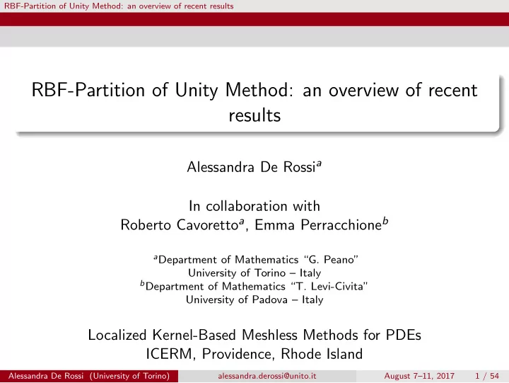
RBF-Partition of Unity Method: an overview of recent results RBF-Partition of Unity Method: an overview of recent results Alessandra De Rossi a In collaboration with Roberto Cavoretto a , Emma Perracchione b a Department of Mathematics G.
RBF-Partition of Unity Method: an overview of recent results RBF-Partition of Unity Method: an overview of recent results Alessandra De Rossi a In collaboration with Roberto Cavoretto a , Emma Perracchione b a Department of Mathematics “G. Peano” University of Torino – Italy b Department of Mathematics “T. Levi-Civita” University of Padova – Italy Localized Kernel-Based Meshless Methods for PDEs ICERM, Providence, Rhode Island Alessandra De Rossi (University of Torino) alessandra.derossi@unito.it August 7–11, 2017 1 / 54
RBF-Partition of Unity Method: an overview of recent results Introduction Acknowledgements This talk gives an overview about the Partition of Unity (PU) interpolation, locally implemented by means of Radial Basis Functions (RBFs), and proposes some original investigations. Other co-authors: Stefano De Marchi (University of Padova, Italy); Greg Fasshauer (Colorado School of Mines, Golden, CO); Gabriele Santin (University of Stuttgart, Germany); Ezio Venturino (University of Torino, Italy). Funds: Department of Mathematics “G. Peano” via the projects “Metodi numerici nelle scienze applicate” (Principal Investigator (PI) A. D.), “Metodi e modelli numerici per le scienze applicate” (PI A. D.), European Cooperation in Science and Technology (ECOST), Gruppo Nazionale per il Calcolo Scientifico (GNCS–INdAM). These researches have been accomplished within RITA (Rete ITaliana di Approssimazione). Alessandra De Rossi (University of Torino) alessandra.derossi@unito.it August 7–11, 2017 2 / 54
RBF-Partition of Unity Method: an overview of recent results Introduction Outline Preliminaries: RBF-PUM interpolation. Improvements of the RBF-PUM: efficiency; accuracy; positivity; stability. Approximation of track data via RBF-PUM. Alessandra De Rossi (University of Torino) alessandra.derossi@unito.it August 7–11, 2017 3 / 54
RBF-Partition of Unity Method: an overview of recent results Preliminaries: RBF-PUM interpolation Essential references Preliminaries: RBF-PUM interpolation I. Babuˇ ska, J.M. Melenk, The partition of unity method , Int. J. Numer. Meth. Eng. 40 (1997), 727–758. M.D. Buhmann, Radial Basis Functions: Theory and Implementation , Cambridge Monogr. Appl. Comput. Math., vol. 12, Cambridge Univ. Press, Cambridge, 2003. G.E. Fasshauer, Meshfree Approximations Methods with Matlab , World Scientific, Singapore, 2007. G.E. Fasshauer, M.J. McCourt, Kernel-based Approximation Methods Using Matlab , World Scientific, Singapore, 2015. H. Wendland, Scattered Data Approximation , Cambridge Monogr. Appl. Comput. Math., vol. 17, Cambridge Univ. Press, Cambridge, 2005. H. Wendland, Fast evaluation of radial basis functions: Methods based on partition of unity , in: C.K. Chui et al. (Eds.), Approximation Theory X: Wavelets, Splines, and Applications, Vanderbilt Univ. Press, Nashville, 2002, 473–483. Alessandra De Rossi (University of Torino) alessandra.derossi@unito.it August 7–11, 2017 4 / 54
RBF-Partition of Unity Method: an overview of recent results Preliminaries: RBF-PU interpolation Statement of the problem Problem Given X N = { x i , i = 1 , . . . , N } ⊆ Ω a set of distinct data points (or data sites or nodes), arbitrarily distributed on a domain Ω ⊆ R M , with an associated set F N = { f i = f ( x i ) , i = 1 , . . . , N } of data values (or measurements or function values), which are obtained by sampling some (unknown) function f : Ω − → R at the nodes x i , the scattered data interpolation problem consists in finding a function R : Ω − → R such that R ( x i ) = f i , i = 1 , . . . , N . Here, we consider RBFs and thus the interpolant is expressed as N � R ( x ) = c k φ ( � x − x k � 2 ) , x ∈ Ω . k =1 Alessandra De Rossi (University of Torino) alessandra.derossi@unito.it August 7–11, 2017 5 / 54
RBF-Partition of Unity Method: an overview of recent results Preliminaries: RBF-PU interpolation Uniqueness of the solution The problem reduces to solving a linear system A c = f , where the entries of A are given by ( A ) ik = φ ( � x i − x k � 2 ) , i , k = 1 , . . . , N . Moreover, the problem is well-posed under the assumption that φ is strictly positive definite. We remark that the uniqueness of the interpolant can be ensured also for the general case of strictly conditionally positive definite functions, by adding a polynomial term. In what follows, we might also refer to the more general case for which Φ : R M × R M − → R is a strictly positive definite kernel, i.e. the entries of A are given by ( A ) ik = Φ ( x i , x k ) , i , k = 1 , . . . , N . Alessandra De Rossi (University of Torino) alessandra.derossi@unito.it August 7–11, 2017 6 / 54
RBF-Partition of Unity Method: an overview of recent results Preliminaries: RBF-PU interpolation Examples of RBFs In Table 1, we summarize several RBFs. Note that r denotes the euclidean distance and ε the shape parameter. Table 1: Examples of RBFs. φ ( r ) = e − ( ε r ) 2 Gaussian C ∞ G φ ( r ) = (1 + ( ε r ) 2 ) − 1 / 2 Inverse MultiQuadric C ∞ IMQ φ ( r ) = e − ε r ern C 0 Mat´ M0 φ ( r ) = e − ε r (1 + ε r ) ern C 2 Mat´ M2 φ ( r ) = e − ε r (3 + 3 ε r + ( ε r ) 2 ) ern C 4 Mat´ M4 φ ( r ) = (1 − ε r ) 2 Wendland C 0 W0 + φ ( r ) = (1 − ε r ) 4 Wendland C 2 + (4 ε r + 1) W2 φ ( r ) = (1 − ε r ) 6 35( ε r ) 2 + 18 ε r + 3 � � Wendland C 4 W4 + Alessandra De Rossi (University of Torino) alessandra.derossi@unito.it August 7–11, 2017 7 / 54
RBF-Partition of Unity Method: an overview of recent results Preliminaries: RBF-PU interpolation Reproducing kernels and Hilbert spaces Definition The space N Φ (Ω) = span { Φ ( · , x ) , x ∈ Ω } , equipped with the bilinear form ( · , · ) H Φ (Ω) defined as � m n � m n � � � � c i Φ ( · , x i ) , d k Φ ( · , x k ) = c i d k Φ ( x i , x k ) . i =1 k =1 i =1 k =1 H Φ (Ω) is known as native space of Φ. Definition The separation and fill distances, which are a measure of data distribution, are respectively given by � � q X N = 1 2 min i � = k � x i − x k � 2 , h X N = sup x k ∈X N � x − x k � 2 min . x ∈ Ω Alessandra De Rossi (University of Torino) alessandra.derossi@unito.it August 7–11, 2017 8 / 54
RBF-Partition of Unity Method: an overview of recent results Preliminaries: RBF-PU interpolation Error bounds for RBF interpolants Theorem Suppose Ω ⊆ R M is open and bounded and satisfies an interior cone condition and let Φ ∈ C 2 k (Ω × Ω) be symmetric and strictly conditionally positive definite of order L. Fix α ∈ N M 0 with | α | ≤ k. Then there exist positive constants h 0 and C independent of x , f and Φ , such that | D α f ( x ) − D α R ( x ) | ≤ Ch k −| α | � C Φ ( x ) | f | N Φ (Ω) , X N provided h X N ≤ h 0 and f ∈ N Φ (Ω) , where � � � � � D β 1 D γ C Φ ( x ) = max max 2 Φ ( w , z ) . � � � | β | + | γ | =2 k w , z ∈ Ω ∩ B ( x , C 2 h X N ) The interpolation with a C 2 k smooth kernel has approximation order k . Alessandra De Rossi (University of Torino) alessandra.derossi@unito.it August 7–11, 2017 9 / 54
RBF-Partition of Unity Method: an overview of recent results Preliminaries: RBF-PU interpolation PUM and regular coverings Dealing with large data sets it is convenient to use the PUM. Its basic idea is to start with a partition of the open and bounded domain Ω into d subdomains or patches Ω j , such that Ω ⊆ ∪ d j =1 Ω j , with some mild overlap among them. Definition Suppose that Ω ⊆ R M is bounded and X N = { x i , i = 1 , . . . , N } ⊆ Ω is given. An open and bounded covering { Ω j } d j =1 is called regular for (Ω , X N ) if the following properties are satisfied: i. for each x ∈ Ω, the number of subdomains Ω j , with x ∈ Ω j , is bounded by a global constant C , ii. each subdomain Ω j satisfies an interior cone condition, iii. the local fill distances h X Nj are uniformly bounded by the global fill distance h X N , where X N j = X N ∩ Ω j . Alessandra De Rossi (University of Torino) alessandra.derossi@unito.it August 7–11, 2017 10 / 54
RBF-Partition of Unity Method: an overview of recent results Preliminaries: RBF-PU interpolation PUM and locally supported weights Definition A family of compactly supported, non-negative and continuous functions { W j } d j =1 is a k -stable partition of unity if i. supp ( W j ) ⊆ Ω j , ii. � d x ∈ Ω , j =1 W j ( x ) = 1 , iii. for every β ∈ N M , with | β | ≤ k , there exists a constant C β > 0 such that C β � � � D β W j L ∞ (Ω j ) ≤ � | β | , j = 1 , . . . , d . � � � � sup x , y ∈ Ω j � x − y � 2 Alessandra De Rossi (University of Torino) alessandra.derossi@unito.it August 7–11, 2017 11 / 54
RBF-Partition of Unity Method: an overview of recent results Preliminaries: RBF-PU interpolation RBF-PUM Then, for each subdomain Ω j we consider a radial basis function R j , as local interpolant and the global approximant is given by: d � I ( x ) = x ∈ Ω . R j ( x ) W j ( x ) , j =1 Thus, to find the PUM interpolant we need to solve d linear systems N j ) T , of the form A j c j = f j , where c j = ( c j 1 , . . . , c j N j ) T and f j = ( f j 1 , . . . , f j ( A j ) ik = φ ( || x j i − x j x j k || 2 ) , i ∈ Ω j , i , k = 1 , . . . , N j . Alessandra De Rossi (University of Torino) alessandra.derossi@unito.it August 7–11, 2017 12 / 54
Recommend
More recommend
Explore More Topics
Stay informed with curated content and fresh updates.

