Space-Time Localized Radial Basis Function Collocation Methods for - - PowerPoint PPT Presentation

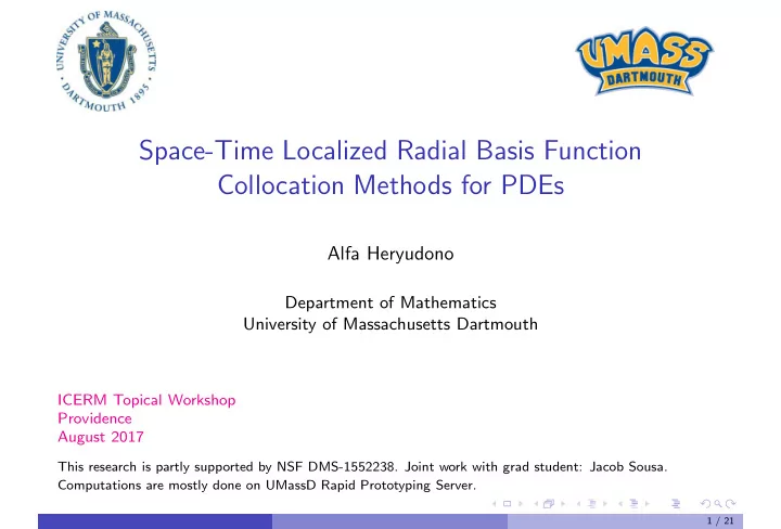
Space-Time Localized Radial Basis Function Collocation Methods for PDEs

Alfa Heryudono

Department of Mathematics University of Massachusetts Dartmouth

ICERM Topical Workshop Providence August 2017

This research is partly supported by NSF DMS-1552238. Joint work with grad student: Jacob Sousa. Computations are mostly done on UMassD Rapid Prototyping Server.

1 / 21

Dealing with Time-Dependent PDEs for RBF Methods

Method of Lines RBF discretization in space + common ODE solver in time. Min changes of PS/FD codes: replace differentiation matrices with RBF versions (Global, RBF-FD, RBF-PU, etc). PS/FD treatments for BCs: Strip-rows, Strip-rows move over columns, fictitious pts/ rect projection (for multiple bcs), penalty, etc. Stability for linear pde case: Eigenvalue and Pseudospectra. Simultaneous Space-Time RBF Boundary value collocation problem in space-time domain. Time is treated as another space variable. RBF-BVP solver have been studied for quite a while. Less worry about choosing ODE solver based on PDE types. Adaptivity, moving boundary, and BCs: same treatments as in BVP cases. No need to rewrite the pde due to var trans (e.g in moving boundary case). Analyzing stability is not clear (e.g. in moving boundary case). Might be expensive to solve (e.g. finding preconditioner, non-linear case).

2 / 21

Space-Time PS Collocation Method: 1D+t linear case

PDE : ut = ux (x, t) ∈ [−1, 1) × (0, T] IC : u(x, 0) = f (x) BC : u(1, t) = g(t) Use PS or Block PS (Driscoll-Fornberg) to create differentiation matrices.

1 0.75 0.5 0.25

• 1
• 1
• 0.5

0.5 1 1

• 1
• 0.5

0.5 1 0.25 0.5 0.75 1 3 / 21

Space-Time PS Collocation Method: 2D+t, linear case

1 0.5 1 1 0.5 2

• 0.5
• 0.5
• 1
• 1

PDE : ut = ∆u + F(x, y, t) (x, y, t) ∈ Ω × (0, T] IC : u(x, y, 0) = f (x, y) BC : u(∂Ω, t) = g(∂Ω, t) kron’s disease is worse in 2D + t case.

1000 2000 3000 4000

nz = 163249

1000 2000 3000 4000 10 20 30 10-14 10-10 10-6 10-2 102 P = symrcm(PLinop); L = gpuArray(Linop(P,P)); PL = gpuArray(PLinop(P,P)); r = gpuArray(rhs(P)); MAXITER = 30; TOL = 1e-14; RESTART = []; [Ugpu,FLAG,RELRES,ITER,RESVEC] = ... gmres(L,r,RESTART,TOL,MAXITER,PL); U(P) = gather(Ugpu); 4 / 21

Space-Time PS Collocation Method: 1D+t, nonlinear case

Human tear film dynamics: 1D model: see H. et. al 2007 ht + qx = 0 on X(t) ≤ x ≤ 1, where q(x, t) = Shxxx h3 3 + βh2

• Boundary conditions

h(X(t), t) = h(1, t) = h0 q(X(t), t) = Xth0 + Qtop q(1, t) = −Qbot.

−1 −0.5 0.5 1 4 8 12

x h(x,t)

t 3.52

Advance the solution in space-time domain: Slab by Slab (Show MATLAB).

5 / 21

RBF-FD Differentiation Matrices

bc bc bc bc bc bc bc bc bc bc bc bc bc bc bc bc bc bc bc bc bc bc bc bc bc bc bc bc bc bc bc bc bc bc bc bc bc bc bc bc bc bc bc bc bc bc bc bc bc bc bc bc bc bc bc bc bc bc bc bc bc bc bc bc bc bc bc bc bc bc bc bc bc bc bc bc bc bc bc bc bc bc bc bc bc bc bc bc bc bc bc bc bc bc bc bc bc bc bc bc

⊕ bc Ω ∂Ω bc bc bc bc bc bc bc bc

⊕

x1 x8 x41 x18 x21 x33 x35 x27 x2 x11

bc bc bc bc bc bc bc bc bc bc bc bc bc bc

sj(x) =

nloc

• k=1

λkφk(x), where φk(x) is a radial basis func- tion centered at xk. Or in Lagrange formulation as sj(x) =

nloc

• k=1

Ψk(x)uk, where Ψ =

• Ψ1(x)

· · · Ψnloc(x)

• =
• φ1(x)

· · · φnloc(x) A−1 , Ψx = Ψ1

x(x)

· · · Ψnloc

x (x)

= φ1

x(x)

· · · φnloc

x (x) A−1

, The matrix A with entries aℓk = φk(x ℓ), ℓ, k = 1, . . . , nloc is local RBF interpolation matrix. BYODM: Bring Your Own Differentiation Matrices

6 / 21

Getting the space-time domain

This is probably for programming on a lazy Sunday: Use Mathematica’s DiscretizeRegion family commands. Surprisingly, Mathematica has many built-in funky domains too. This is also useful if you want to compare results with finite-element.

R = ImplicitRegion[-0.6 Sin[t] <= x, {{x, -1, 1}, {t, 0, 1.5 Pi}}]; ev = DiscretizeRegion[R]; pts = MeshCoordinates[ev]; Export["spacetimedom.mat", pts];

To obtained boundary points, you can use Mathematica or boundary command in MATLAB.

7 / 21

t+1D Advection Example

PDE : ut = ux (x, t) ∈ [X(t), 1) × (0, T] IC : u(x, 0) = f (x) BC : u(1, t) = g(t)

IMQ-RBF:

1

√

1+(εr)2 . r2 = (x − xi)2 + (t − ti)2

solution in space-time domain f (x) = e−10(x−0.15+0.35y)2 , g(t) = 0

Dt − Dx I u = f g

P = symrcm(L); u(P) = L(P,P)\RHS(P);

• r

MAXITER = 20; TOL = 1e-13; RESTART = []; [ML,MU] = ilu(L(P,P),struct(’type’,’ilutp’,’droptol’,1e-6)); u(P) = gmres(L(P,P),RHS(P),RESTART,TOL,MAXITER,ML,MU); portion of system matrix after applying MATLAB symrcm 8 / 21

t+1D Advection Example

PDE : ut = ux + F(x, t) (x, t) ∈ [X(t), 1) × (0, T] IC : u(x, 0) = f (x) BC : u(1, t) = g(t)

IMQ-RBF:

1

√

1+(εr)2 . r2 = (x − xi)2 + (t − ti)2

Get RBF-QR diffmat from Elisabeth’s website.

solution in space-time domain f (x) = e−10(x−0.15+0.35y)2

Dt − Dx I u = F f g

10 20 30 40 50 10

−5

10

−4

10

−3

10

−2

10

−1

10

−4.1

√ N ||.||∞

nloc = 50, ε=3 Test case 1 Test case 2 Test case 3 Test case 4 5 10 15 10-8 10-7 10-6 10-5 10-4 10-3 10-2 10-1

||.||

slope = -1.227

8 / 21

t+1D Advection with Variable Speed Example

PDE : ut = a(x, t)ux + F(x, t) (x, t) ∈ [X(t), 1) × (0, T] IC : u(x, 0) = f (x) BC : u(1, t) = g(t) a(x, t) = exp((1 + t)(1 + cos(3x))

Bribe Varun for PHS diffmat.

solution in space-time domain f (x) = e−10(x−0.15+0.35y)2

Dt − diag(a)Dx I u = F f g

10 20 30 40 50 10

−5

10

−4

10

−3

10

−2

10

−1

10

−4.1

√ N ||.||∞

nloc = 50, ε=3 Test case 1 Test case 2 Test case 3 Test case 4 5 10 15 10-8 10-7 10-6 10-5 10-4 10-3 10-2 10-1

||.||

slope = -1.456

9 / 21

Analyzing Stability ?

Let’s take a look at one step ( 2 levels) space-time global RBF method. a x1 x2 ∆x . . . xj . . . xn−1 xn b t x′

1

x′

2

. . . x′

j

. . . x′

n−1

x′

n

t + ∆t for a simple 1-D advection equation PDE: ∂u ∂t = ∂u ∂x for x ∈ [a, b) IC: u(x, 0) = u0(x) when t = 0 BC: u(b, t) = g(t) at x = b u(x) =

n

• j=1

λjφ(εx − xj) +

n

• j=1

λ′

jφ(εx − x′ j ),

where {xj} and {xj} are centers at the old time level and new time level respectively.

10 / 21

a x1 x2 ∆x . . . xj . . . xn−1 xn b t x′

1

x′

2

. . . x′

j

. . . x′

n−1

x′

n

t + ∆t Our goal is to find the unknowns {λj} and {λ′

j}. This can be done by enforcing

initial and boundary data and satisfying the PDE at the interior points that lead to solving system of linear equations

          

A B C D

                      λ1 . . . λn λ′

1

. . . λ′

n

           =            uo(x1) . . . uo(xn) . . . g(t)           

11 / 21

          

A B C D

                      λ1 . . . λn λ′

1

. . . λ′

n

           =            uo(x1) . . . uo(xn) . . . g(t)           

The block matrices A, B, C, D are all n × n matrices with elements: Aij = φ(εxi − xj) Bij = φ(εxi − x′

j )

Cij = Lφ(εx′

i − xj)

Dij = Lφ(εx′

i − x′ j )

for all i, j = 1, · · · , n and L := ∂

∂t − ∂ ∂x . The last row C and D must be slightly

modified to satisfy the boundary condition at x′

n = b.

12 / 21

Amplification Matrix and Stability Region

The process of marching in time to the new time level is given by

   u(x′

1)

. . . u(x′

n)

   =   G      u(x1) . . . u(xn)    where G = B A A B C D −1 I

• ,

and I is an n × n identity matrix. The method is numerically stable if spectral radius ρ(G) < 1.

log(∆ t / ∆ x) −log(ε) −4 −3 −2 −1 1 −6 −5 −4 −3 −2 −1 0.5 1 1.5 2

IMQ, g(t) = 0, N = 50: to avoid blowing up the solution, the ratio of ∆t/∆x vs shape parameter ε must be away from the darker alley in the the stability region, i.e we want to avoid ρ(G) ≥ 1

13 / 21

Adaptivity for BVP based on Residual subsampling

1

Initial coarse collection of nonoverlapping regular boxes in Rd that cover the domain Ω of interest.

2

Geometric adaptation.

3

Refining and Coarsening steps.

2D initial boxes

−1 −0.75 −0.5 −0.25 0.25 0.5 0.75 1 −1 −0.75 −0.5 −0.25 0.25 0.5 0.75 1

x y

1D initial boxes

−1 −0.75 −0.5 −0.25 0.25 0.5 0.75 1

x

Irregular geometry

−1 −0.5 0.5 1 −1 −0.5 0.5 1 x y

see Driscoll & H (2007)

14 / 21

Rules of refining and coarsening centers

Refinement strategy: converting all check points if any of them have residual errors are greater than θr described as ⊗ into RBF centers as dots and remove its parent. Coarsening strategy: reactivate all RBF cen- ters if all of its grand children have residual errors less than θc described as ⊗. a layout of quadtree. With this rule, centers are located as leaves.

15 / 21

Depth first search algorithm

Pruning device to save computing pairwise distances.:O(nq log(N)) instead of O(N) per query point. Partial updates for lists of neighbors. Embarassingly parallel neighbors’ search.

Values at × are computed using local RBF interpolant of the box whose midpoint is the parent node of the check points. Uniform nodes distribution

10

1

10

2

10

3

10

4

10

5

10

1

10

2

10

3

10

4

10

5

N average distance computations

N nq log4N

Some non-uniform nodes distribution

10

1

10

2

10

3

10

4

10

5

10

1

10

2

10

3

10

4

10

5

N average distance computations

N nq log4 N

16 / 21

t+1D Nonlinear Example

Burgers’ Equation

υuxx − uux = ut, 0 < x < 1 u(0, t) = u(1, t) = 0 u(x, 0) = sin(2πx) + 1

2sin(πx).

where, υ = 10−3 MATLAB’s fsolve is used to solve the nonlinear

• system. Jacobian file is provided.

0.5 1 0.1 0.2 −1 −0.5 0.5 1 1.5

t x

0.5 1 0.1 0.2 −1 −0.5 0.5 1 1.5

t x

0.5 1 0.1 0.2 −1 −0.5 0.5 1 1.5

t x

0.5 1 0.1 0.2 −1 −0.5 0.5 1 1.5

x t

N = 485

17 / 21

Dealing with Multiple Boundary Conditions

PDE : Tear film PDE in terms of h (x, t) ∈ [X(t), 1) × (0, T] IC : h(x, 0) = f (x) BC : h(1, t) = h(X(t), t) = h0 hxxx(1, t) = g1(t) hxxx(X(t), t) = g2(X(t), t)

−0.2 0.2 0.6 1 0.5 1 1.5 4 8 12 16

t x h(x,t)

2 4 6 8 10 12

PDE : ht = Sqx ,S is a constant q = nonlinear flux (x, t) ∈ [X(t), 1) × (0, T] IC : h(x, 0) = f (x) BC : h(1, t) = h(X(t), t) = h0 q(1, t) = g1(t) q(X(t), t) = g2(X(t), t)

18 / 21

t+2D Advection Example

ut = 0.5ux + 0.75uy + F(x, y, t) (x, y) ∈ [0, 1) × [0, 1) u(1, y, t) = f1(1, y, t) u(x, 1, t) = f2(x, 1, t) u(x, y, 0) = g(x, y)

6 8 12 10

−5

10

−4

10

−3

10

−2

10

−1

−5.2

N 1/3 Error

nloc = 105, ε=0.75 Test case 1 Test case 2

19 / 21

t+2D Wave Example

utt = ∆u (x, y) ∈ (0, 1) × (0, 1) u(x, y, t) = 0 at the boundary u(x, y, 0) = g(x, y) ut(x, y, 0) = 0

extra ghost/fictitious points for enforcing ut

20 / 21

On-going study or future questions

Stability: Can it only be done through adaptivity ? Least-Squares Space-time RBF-PU might be worth to try. Adaptivity in terms of partitions. Move away from points adaptivity. Preconditioner ? Possible GR application. Application to 2D + t Human Tear Film Dynamics. Enforce my grad students to finish the papers.

y x y x x y x y Fully open 2/3 open 1/3 open Closed

======================

21 / 21