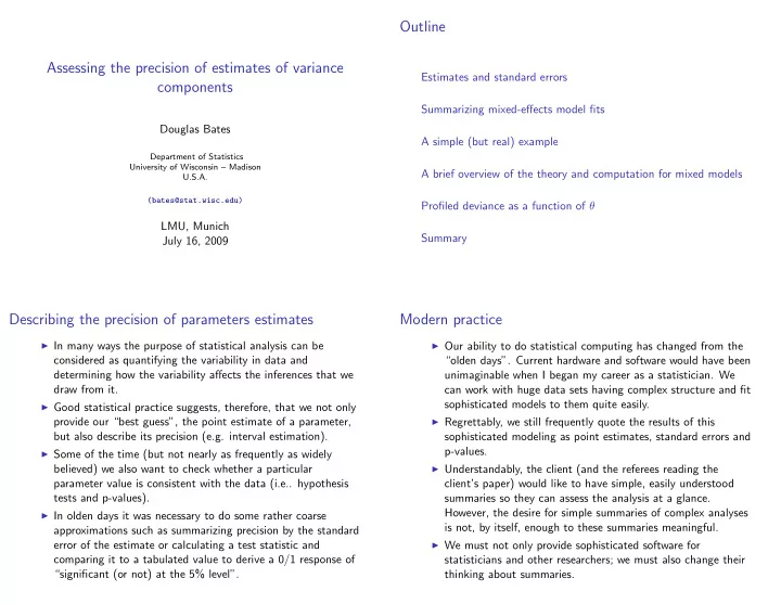
Outline Assessing the precision of estimates of variance Estimates - PowerPoint PPT Presentation

Outline Assessing the precision of estimates of variance Estimates and standard errors components Summarizing mixed-effects model fits Douglas Bates A simple (but real) example Department of Statistics University of Wisconsin – Madison A brief overview of the theory and computation for mixed models U.S.A. (bates@stat.wisc.edu) Profiled deviance as a function of θ LMU, Munich Summary July 16, 2009 Describing the precision of parameters estimates Modern practice ◮ In many ways the purpose of statistical analysis can be ◮ Our ability to do statistical computing has changed from the considered as quantifying the variability in data and “olden days”. Current hardware and software would have been determining how the variability affects the inferences that we unimaginable when I began my career as a statistician. We draw from it. can work with huge data sets having complex structure and fit sophisticated models to them quite easily. ◮ Good statistical practice suggests, therefore, that we not only ◮ Regrettably, we still frequently quote the results of this provide our “best guess”, the point estimate of a parameter, but also describe its precision (e.g. interval estimation). sophisticated modeling as point estimates, standard errors and p-values. ◮ Some of the time (but not nearly as frequently as widely ◮ Understandably, the client (and the referees reading the believed) we also want to check whether a particular parameter value is consistent with the data (i.e.. hypothesis client’s paper) would like to have simple, easily understood tests and p-values). summaries so they can assess the analysis at a glance. However, the desire for simple summaries of complex analyses ◮ In olden days it was necessary to do some rather coarse is not, by itself, enough to these summaries meaningful. approximations such as summarizing precision by the standard ◮ We must not only provide sophisticated software for error of the estimate or calculating a test statistic and comparing it to a tabulated value to derive a 0/1 response of statisticians and other researchers; we must also change their “significant (or not) at the 5% level”. thinking about summaries.

Summaries of mixed-effects models What does a standard error tell us? ◮ Commercial software for fitting mixed-effects models (SAS ◮ Typically we use a standard error of a parameter estimate to PROC MIXED, SPSS, MLwin, HLM, Stata) provides assess precision (e.g. a 95% confidence interval on µ is estimates of fixed-effects parameters, standard errors, degrees x ± 2 s roughly ¯ √ n ) or to form a test statistic (e.g. a test of of freedom and p-values. They also provide estimates of ¯ x H 0 : µ = 0 versus H a : µ � = 0 based on the statistic s/ √ n ). variance components and standard errors of these estimates. ◮ The mixed-effects packages for R that I have written ( nlme ◮ Such intervals or test statistics are meaningful when the with Jos´ e Pinheiro and lme4 with Martin M¨ achler) do not distribuion of the estimator is more-or-less symmetric. provide standard errors of variance components. lme4 doesn’t ◮ We would not, for example, quote a standard error of � σ 2 even provide p-values for the fixed effects. because we know that the distribution of this estimator, even ◮ This is a source of widespread anxiety. Many view it as an in the simplest case (the mythical i.i.d. sample from a indication of incompetence on the part of the developers Gaussian distribution), is not at all symmetric. We use (“Why can’t lmer provide the p-values that I can easily get quantiles of the χ 2 distribution to create a confidence interval. from SAS?”) ◮ Why, then, should we believe that when we create a much ◮ The 2007 book by West, Welch and Galecki shows how to use more complex model the distribution of estimators of variance all of these software packages to fit mixed-effects models on 5 components will magically become sufficiently symmetric for different examples. Every time they provide comparative standard errors to be meaningful? tables they must add a footnote that lme doesn’t provide standard errors of variance components. The Dyestuff data set Dyestuff data plot ◮ The Dyestuff , Penicillin and Pastes data sets all come from the classic book Statistical Methods in Research and Production , edited by O.L. Davies and first published in 1947. E ● ● ● ● ● ◮ The Dyestuff data are a balanced one-way classification of C ● ● ● ● ● ● ● B ● ● Batch ● the Yield of dyestuff from samples produced from six A ● ● ● ● ● Batch es of an intermediate product. See ?Dyestuff . D ● ● ● ● ● > str(Dyestuff) ● ● F ● ● ● ’data.frame’: 30 obs. of 2 variables: 1450 1500 1550 1600 Yield of dyestuff (grams of standard color) $ Batch: Factor w/ 6 levels "A","B","C","D",..: 1 1 1 1 1 2 2 2 2 2 ... $ Yield: num 1545 1440 1440 1520 1580 ... > summary(Dyestuff) ◮ The line joins the mean yields of the six batches, which have Batch Yield been reordered by increasing mean yield. A:5 Min. :1440 ◮ The vertical positions are jittered slightly to reduce B:5 1st Qu.:1469 overplotting. The lowest yield for batch A was observed on C:5 Median :1530 D:5 Mean :1528 two distinct preparations from that batch. E:5 3rd Qu.:1575 F:5 Max. :1635

A mixed-effects model for the dyestuff yield REML estimates versus ML estimates > fm1 <- lmer(Yield ~ 1 + (1 | Batch), Dyestuff) ◮ The default parameter estimation criterion for linear mixed > print(fm1) models is restricted (or “residual”) maximum likelihood (REML). Linear mixed model fit by REML Formula: Yield ~ 1 + (1 | Batch) ◮ Maximum likelihood (ML) estimates (sometimes called “full Data: Dyestuff maximum likelihood”) can be requested by specifying REML = AIC BIC logLik deviance REMLdev FALSE in the call to lmer . 325.7 329.9 -159.8 327.4 319.7 Random effects: ◮ Generally REML estimates of variance components are Groups Name Variance Std.Dev. preferred. ML estimates are known to be biased. Although Batch (Intercept) 1764.0 42.00 REML estimates are not guaranteed to be unbiased, they are Residual 2451.3 49.51 Number of obs: 30, groups: Batch, 6 usually less biased than ML estimates. Fixed effects: ◮ Roughly, the difference between REML and ML estimates of Estimate Std. Error t value variance components is comparable to estimating σ 2 in a (Intercept) 1527.50 19.38 78.81 fixed-effects regression by SSR / ( n − p ) versus SSR /n , where ◮ Fitted model fm1 has one fixed-effect parameter, the mean SSR is the residual sum of squares. yield, and one random-effects term, generating a simple, ◮ For a balanced, one-way classification like the Dyestuff data, scalar random effect for each level of Batch . the REML and ML estimates of the fixed-effects are identical. Re-fitting the model for ML estimates Evaluating the deviance function ◮ The profiled deviance function for such a model can be expressed as a function of 1 parameter only, the ratio of the > (fm1M <- update(fm1, REML = FALSE)) random effects’ standard deviation to the residual standard Linear mixed model fit by maximum likelihood deviation. Formula: Yield ~ 1 + (1 | Batch) ◮ A very brief explanation is based on the n -dimensional Data: Dyestuff response random variation, Y , whose value, y , is observed, AIC BIC logLik deviance REMLdev 333.3 337.5 -163.7 327.3 319.7 and the q -dimensional, unobserved random effects variable, B , Random effects: with distributions Groups Name Variance Std.Dev. � � Zb + Xβ , σ 2 I n Batch (Intercept) 1388.4 37.261 ( Y | B = b ) ∼ N B ∼ N ( 0 , Σ θ ) , , Residual 2451.2 49.510 ◮ For our example, n = 30 , q = 6 , X is a 30 × 1 matrix of 1 s, Number of obs: 30, groups: Batch, 6 Fixed effects: Z is the 30 × 6 matrix of indicators of the levels of Batch and Estimate Std. Error t value Σ is σ 2 b I 6 . (Intercept) 1527.50 17.69 86.33 ◮ We never really form Σ θ ; we always work with the relative (The extra parentheses around the assignment cause the value to covariance factor , Λ θ , defined so that be printed. Generally the results of assignments are not printed.) Σ θ = σ 2 Λ θ Λ ⊺ θ . In our example θ = σ b σ and Λ θ = θ I 6 .