[PPT] - Option Pricing with Semi-Markov Switching Lvy Process Financial PowerPoint Presentation

SLIDE 1

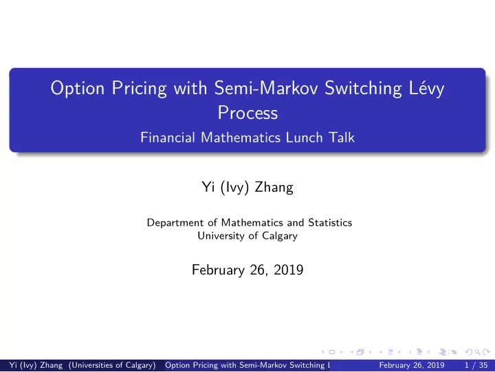
Option Pricing with Semi-Markov Switching Lévy Process

Financial Mathematics Lunch Talk Yi (Ivy) Zhang

Department of Mathematics and Statistics University of Calgary

February 26, 2019

Yi (Ivy) Zhang (Universities of Calgary) Option Pricing with Semi-Markov Switching Lévy Process February 26, 2019 1 / 35

SLIDE 2

Markov Chains

Markov Chain: a stochastic process that satisfies the "Markov Property" Markov Property: the "memoryless" property - the conditional probability distribution of future states of the process (conditional on both past and present states) depends only upon the present state, not on the sequence of events that preceded it

Yi (Ivy) Zhang (Universities of Calgary) Option Pricing with Semi-Markov Switching Lévy Process February 26, 2019 2 / 35

SLIDE 3

Semi-Markov Chains

Consider a state space S = {1, 2, ..., N} and a set of random variables (Xn, τn), where τn are the jump times and Xn are the associated states in the Markov Chain. The inter-arrival times are defined by θn = τn − τn−1. Then the sequence (Xn, τn) is called a Markov Renewal Process if Pr(θn+1 ≤ t, Xn+1 = j|(X0, τ0), (X1, τ1), ..., (Xn = i, τn)) =Pr(θn+1 ≤ t, Xn+1 = j|Xn = i)∀n ≥ 1, t ≥ 0, i, j ∈ S

Yi (Ivy) Zhang (Universities of Calgary) Option Pricing with Semi-Markov Switching Lévy Process February 26, 2019 3 / 35

SLIDE 4

Markov and semi-Markov Processes

Semi-Markov Process: Define a new stochastic process Yt := Xn for t ∈ [τn, τn+1], then Yt is called a semi-Markov process. If the inter-arrival times in a semi-Markov process are exponentially distributed, then we have a continuous-time Markov chain, i.e. Pr(θn+1 ≤ t, Xn+1 = j|Xn = i) = Pr(Xn+1 = j|Xn = i)(1 − eλit) For semi-Markov processes, the inter-arrival times can be from any arbitrary distribution.

Yi (Ivy) Zhang (Universities of Calgary) Option Pricing with Semi-Markov Switching Lévy Process February 26, 2019 4 / 35

SLIDE 5

Why Semi-Markov Switching Process?

To price financial derivatives, we often use St = S0eLt where Lt is the semi-Markov switching process in our case. Many previous literatures are mainly using Markov switching models, ex. Buffington and Elliott. Because of the memoryless property of a Markov process, it is argued that a semi-Markov model is more adequate to model pricing on a financial market. We will focus on semi-Markov switching models where the distribution of holding times is Gamma distributed.

Yi (Ivy) Zhang (Universities of Calgary) Option Pricing with Semi-Markov Switching Lévy Process February 26, 2019 5 / 35

SLIDE 6

Gamma Distribution

k: shape parameter; θ: scale parameter pdf: fG(x) = θk Γ(k)xk−1e−θx x > 0 characteristic function: φGamma(u; k, θ) =

1 − iu

θ

−k

Mean and Variance: E[X] = k/θ Var(X) = k/θ2

Yi (Ivy) Zhang (Universities of Calgary) Option Pricing with Semi-Markov Switching Lévy Process February 26, 2019 6 / 35

SLIDE 7

Gamma vs Exponential Distributions

Why Gamma?

To model the holding times of semi-Markov regime switching process X;
Easy to compare with the Markov case where the exponential distribution

is just a special case of gamma distribution with k = 1.

Figure: PDFs of Gamma vs Exponential

Yi (Ivy) Zhang (Universities of Calgary) Option Pricing with Semi-Markov Switching Lévy Process February 26, 2019 7 / 35

SLIDE 8

Lévy Process

A cádlág, adapted, real valued stochastic process L = (Lt)t≥0 with L0 = 0 is a Lévy process if the following conditions are satisfied: (i)L has independent increments, i.e. Lt − Ls is independent of Fs for any 0 ≤ s ≤ t ≤ T. (ii) L has stationary increments, i.e. the distribution of Lt+s − Lt does not depend on t for any s, t ≥ 0. (iii) L is stochastically continuous, i.e. for every t ≥ 0 and ǫ > 0: lims→tP(|Lt − Ls| > ǫ) = 0 Examples of Lévy processes: Brownian motion, Poisson process, Variance Gamma process

Yi (Ivy) Zhang (Universities of Calgary) Option Pricing with Semi-Markov Switching Lévy Process February 26, 2019 8 / 35

SLIDE 9

Variance Gamma as the Lévy Process

We will then introduce the Variance Gamma process as the Lévy process that is dominating the pricing process within each regime. Characteristic function of the VG(σ, ν, θ) law: φ(u; σ, ν, θ) =

1 − iuθν + 1

2σ2νu2−1/ν Characteristic function of the VG process: E[eiuLVG

t ] = φVG(u; σ

√ t, ν/t, tθ) = (φVG(u; σ, ν, θ))t =

1 − iuθν + 1

2σ2νu2−t/ν E[Lt] = θt, Var(Lt) = σ2t + θ2νt.

Yi (Ivy) Zhang (Universities of Calgary) Option Pricing with Semi-Markov Switching Lévy Process February 26, 2019 9 / 35

SLIDE 10

Characteristic Function under Risk-Neutral measure

Introduction

Under the risk-neutral measure P: φRN(u) = exp

i∆ut − t

ν ln

1 − iuθν + 1

2σ2u2ν

= ei∆ut1 − iuθν + 1

2σ2u2ν

−t/ν

where ∆ is the risk-neutral drift and equal to ∆ = r + ln(1 − θν − 1

2σ2ν)

ν r: risk-neutral rate

Yi (Ivy) Zhang (Universities of Calgary) Option Pricing with Semi-Markov Switching Lévy ProcessFebruary 26, 2019 10 / 35

SLIDE 11

Semi-Markov Switching Lévy Processes

Introduction

The semi-Markov switching Lévy process is defined as Lt = Lj

t,

Xt = ej, Lj

t: Lévy process

Xt: finite state semi-Markov switching process E = {e1, e2, ..., em}: state space

Yi (Ivy) Zhang (Universities of Calgary) Option Pricing with Semi-Markov Switching Lévy ProcessFebruary 26, 2019 11 / 35

SLIDE 12

Semi-Markov Switching Lévy Processes

Now, we will introduce some definitions and notations: 0 < t1 < t2 < t3...: jump times for X Qi,j(t) = P(Xn = j, tn − tn−1 ≤ t|Xn−1 = i) pij = lim

t→∞ Qi,j(t)

F(t|i, j) = P(τn ≤ t|Xn = j, Xn−1 = i) S(t|i, j) = 1 − F(t|i, j) λi,j(t) = pi,j −dS

dt (t|i, j)

S(t−|i)

Yi (Ivy) Zhang (Universities of Calgary) Option Pricing with Semi-Markov Switching Lévy ProcessFebruary 26, 2019 12 / 35

SLIDE 13

Semi-Markov Switching Lévy Processes

The Lévy-Itô decomposition for Lj

t has the following form:

Lj

t = ajt + σjWt +

|z|>1

zNj(t, dz) +

|z|≤1

z(Nj(t, dz) − mj(dz)t). W : Brownian motion; N: random measure counting the jumps; m(dz): compensated measure/Lévy measure: expected number of jumps. The triplet (aj, σj, mj(dz)) is completely determined by the characteristic function of Lj

t:

φj

t(u) = E[eiuLj

t]

= exp{t(iaju − 1 2σ2

j u2 +

R

(eiuz − 1 − iz1(|z| ≤ 1))mj(dz))}

Yi (Ivy) Zhang (Universities of Calgary) Option Pricing with Semi-Markov Switching Lévy ProcessFebruary 26, 2019 13 / 35

SLIDE 14

Itô’s Formula for Semi-Markov Switching Lévy Processes

Considering the following SDE: dxt = xtdLj

t,

x(tn) = xn, t ∈ [tn, tn+1) Also define: γt =

n≥0

(t − tn)1tn≤t<tn+1 αn: state jump process caused by the semi-Markov process ln(αn): jump in log price at regime change g: density function of αn ˜ g(z|Xn−1, Xn) = g(ez|Xn−1, Xn)ez µ(t, A, B) =

n≥1

1(t≥tn,ln(αn)∈A,(Xn−1,Xn)∈B) ν(t, A, {i, j}) =

t

z∈A

˜ g(z|i, j)λi,j(γs)dzds

Yi (Ivy) Zhang (Universities of Calgary) Option Pricing with Semi-Markov Switching Lévy ProcessFebruary 26, 2019 14 / 35

SLIDE 15

Itô’s Formula for Semi-Markov Switching Lévy Processes

dV (s, γs, Xs, xs) =(LV )(s, γs, Xs, xs)ds + σjxs ∂V ∂x dWs +

|z|≤1
V (s, γs, Xs, xs + xsGj(z)) − V (s, γs, Xs, xs)

˜

Nj(ds, dz) +

|z|>1
V (s, γs, Xs, xs + xsHj(z)) − V (s, γs, Xs, xs)

˜

Nj(ds, dz) +

z∈R
j∈E\{Xs}
V (s, γs, j, xsez) − V (s, γs, Xs, xs)
˜

µ(ds, dz, {(Xs, j)})

Yi (Ivy) Zhang (Universities of Calgary) Option Pricing with Semi-Markov Switching Lévy ProcessFebruary 26, 2019 15 / 35

SLIDE 16

Itô’s Formula for Semi-Markov Switching Lévy Processes

where (LV )(s, γs, Xs, xs) =∂V ∂s + ∂V ∂γ + ajxs− ∂V ∂x + 1 2σ2

j x2 s

∂2V ∂x2 +

|z|≤1
V (s, γs, Xs, xs + xsGj(z) − V (s, γs, Xs, xs) − Gj(z)xs

∂V ∂x

mj(dz)

+

|z|>1
V (s, γs, Xs, xs + xsHj(z)) − V (s, γs, Xs, xs)
mj(dz)

+

z∈R
j=Xs

λXs,j(γs)

V (s, γs, j, xsez) − V (s, γs, Xs, xs)
˜

g(z|Xs, j)dz G(z), H(z): smooth functions defining the jump size z.

Yi (Ivy) Zhang (Universities of Calgary) Option Pricing with Semi-Markov Switching Lévy ProcessFebruary 26, 2019 16 / 35

SLIDE 17

Characteristic Function for Semi-Markov Switching Lévy Processes

Our goal here is to derive a closed form expression for the conditional characteristic function Φ(u, t, γ, j, x) = E

eiu ln(xt)
γ0 = γ, X0 = j, x0 = x
for the log price process below

ln(xt) =

n(t)

a=1

ln(αa) + Lj

t.

Yi (Ivy) Zhang (Universities of Calgary) Option Pricing with Semi-Markov Switching Lévy ProcessFebruary 26, 2019 17 / 35

SLIDE 18

Characteristic Function for Semi-Markov Switching Lévy Processes

The closed form expression for the conditional characteristic vector function of ln(x) is Φ(u, t, γ, x) = exp[iu ln(x)] exp

t+γ

γ

M(u, s)ds

.1

where i = √−1, Φ(u, t, γ, x) is an m-dimensional column vector with the k-th component Φ(u, t, γ, k, x) for k ∈ E. Mq,p(u, γ) = iua(q) − 1 2σ2(q)u2 +

|z|≤1

[eiuG(z,q) − 1 − iuG(z, q)]m(q, dz) +

|z|>1

[eiuH(z,q) − 1]m(q, dz) + λq,q(γ), if p = q, = λq,p(γ)

z∈R

eiuz ˜ g(z|q, p)dz,

therwise.

Assuming [M(u, γ1), M(u, γ2)] = 0

Yi (Ivy) Zhang (Universities of Calgary) Option Pricing with Semi-Markov Switching Lévy ProcessFebruary 26, 2019 18 / 35

SLIDE 19

Examples of Semi-Markov Switching Lévy Processes

Semi-Markov Black Scholes Process

dxt = xt[ajdt + σjdWt], x(tn) = xn, t ∈ [tn, tn+1) The matrix M found within the closed form characteristic function is Mq,p(u, γ) =iua(q) − 1 2σ2(q)u2 + λq,q(γ), if p = q λq,p(γ)

z∈R

eiuz ˜ g(z|q, p)dz,

therwise

Yi (Ivy) Zhang (Universities of Calgary) Option Pricing with Semi-Markov Switching Lévy ProcessFebruary 26, 2019 19 / 35

SLIDE 20

Examples of Semi-Markov Switching Lévy Processes

Semi-Markov Merton Jump Diffusion Process

dxt = xt[ajdt + σjdWt +

z∈R

zmj(dz, dt)], x(tn) = xn, t ∈ [tn, tn+1) The matrix M found within the closed form characteristic function is Mq,p(u, γ) =iu[a(q) −

|z|≤1

zmq(dz)] − 1 2σ2(q)u2 +

z∈R

[eiuz − 1]mq(dz) + λq,q(γ), if p = q λq,p(γ)

z∈R

eiuz ˜ g(z|q, p)dz,

therwise

Yi (Ivy) Zhang (Universities of Calgary) Option Pricing with Semi-Markov Switching Lévy ProcessFebruary 26, 2019 20 / 35

SLIDE 21

Option Pricing using FRFT

Carr and Madan’s Method with FRFT

Let sT := ln(ST) and k := ln(K), where K is the strike price of the

ption. Then we know that the value of a European call option with

maturity T as a function of k is given by CT(k) =

∞

k

e−rT(es − ek)qT(s)ds where qT(s) is the risk-neutral density function of s. Define a modified call price function: cT(k) = eαkCT(k), α > 0.

Yi (Ivy) Zhang (Universities of Calgary) Option Pricing with Semi-Markov Switching Lévy ProcessFebruary 26, 2019 21 / 35

SLIDE 22

Option Pricing using FRFT

Fourier Transform

The Fourier transform of cT(k) is then given by FcT (u) = ψT(u) =

∞

−∞

eiukcT(k)dk and the inverse Fourier transform of cT(k) is given by cT(k) = 1 2π

∞

−∞

e−iukFcT (u)du = 1 2π

∞

−∞

e−iukψT(u)du So that CT(k) = e−αkcT(k) = e−αk 1 2π

∞

−∞

e−iukψT(u)

Yi (Ivy) Zhang (Universities of Calgary) Option Pricing with Semi-Markov Switching Lévy ProcessFebruary 26, 2019 22 / 35

SLIDE 23

Option Pricing using FRFT

We obtain CT(k) = e−αk π

∞

e−iukψT(u)du Carr and Madan obtained the analytic form for ψT(u) below ψT(u) = e−rTφT(u − (α + 1)i) α2 + α − u2 + i(2α + 1)u

Yi (Ivy) Zhang (Universities of Calgary) Option Pricing with Semi-Markov Switching Lévy ProcessFebruary 26, 2019 23 / 35

SLIDE 24

FFT

The FFT method is basically approximating the continuous Fourier transform with its discrete counterpart

∞

e−ixuh(u)du ≈

N−1

j=0

e−i 2π

N kjhj

k = 0, ..., N − 1 Using the Trapezoidal Rule as one of the integration rules, we can get

∞

e−iukψ(u)du ≈

N−1

j=0

e−iujkψ′(uj)η η: discretization step/grid spacing

Yi (Ivy) Zhang (Universities of Calgary) Option Pricing with Semi-Markov Switching Lévy ProcessFebruary 26, 2019 24 / 35

SLIDE 25

FFT

Since the sum is not a direct application of the FFT algorithm, we will take log-strikes ranging from −b to b, where b = 1

2Nλ: N−1

j=0

e−iujkvψ′(uj)η =

N−1

j=0

e−iuj(− 1

2 Nλ+λv)ψ′(uj)η

=

N−1

j=0

e−iηjλveiηj Nλ

2 ψ′(uj)η

If we set hj = eiηj Nλ

2 ψ′(uj)η and ηλ = 2π

N , then we can rewrite the

summation as the following:

N−1

j=0

e−i 2π

N jvhj Yi (Ivy) Zhang (Universities of Calgary) Option Pricing with Semi-Markov Switching Lévy ProcessFebruary 26, 2019 25 / 35

SLIDE 26

Fractional FFT

FRFT

The Fractional FFT is an easy and fast way to compute sums in the form

f

N−1

j=0

e−i2πkjǫhj FFT is just a special case of FRFT where ǫ = 1

N .

1. Choose the initial parameters, the number of points N, the upper

integration bound a and the bound for log prices b (ranging from e−b to eb).

2. The integration grid spacing is then given by η = a/N, the log-strikes

grid spacing λ = 2b/N and the fractional parameter ǫ = ηλ.

3. The input grid is spanned on the interval (a, N) with grid spacing λ and

the output grid on the interval (−b, b) with grid spacing λ.

Yi (Ivy) Zhang (Universities of Calgary) Option Pricing with Semi-Markov Switching Lévy ProcessFebruary 26, 2019 26 / 35

SLIDE 27

Option Pricing

For Xs = j, the Q risk-neutral option price C satisfies the following PIDE: LV (s, T, K, γs, j, xs) = 0 V (T, T, K, yT, XT, xT) = e

T

0 ruduS(xT, K)

and V (s, T, K, γs, j, xs) = e

s

0 ruduC(s, T, K, γs, j, xs).

Moreover, the vector solution C(s, T, K, γ, x) = (C(s, T, K, γ, 1, x), ..., C(s, T, K, γ, m, x)) has the Fourier Transform with respect to ln(x) below: ˜ C(s, T, K, γ, w) =< exp

T−t+γ

γ

M(u, s)ds

.[˜

S(w).ej], 1 > . L: infinitesimal generator

Yi (Ivy) Zhang (Universities of Calgary) Option Pricing with Semi-Markov Switching Lévy ProcessFebruary 26, 2019 27 / 35

SLIDE 28

Simulation Results

(a) Regime 1 (b) Regime 2 Figure: Effect of Shape Parameter on Markov vs semi-Markov Option Prices

Yi (Ivy) Zhang (Universities of Calgary) Option Pricing with Semi-Markov Switching Lévy ProcessFebruary 26, 2019 28 / 35

SLIDE 29

Simulation Results

Figure: Effects of the Shape Parameter on the Implied Volatility

Yi (Ivy) Zhang (Universities of Calgary) Option Pricing with Semi-Markov Switching Lévy ProcessFebruary 26, 2019 29 / 35

SLIDE 30

Calibration

Figure: DJIA and NASDAQ European Call Option Quotes

Yi (Ivy) Zhang (Universities of Calgary) Option Pricing with Semi-Markov Switching Lévy ProcessFebruary 26, 2019 30 / 35

SLIDE 31

Gradient Descent

Goal: to minimize

N

i=1

(cMarket

i

− cModel

i,θ

)2. If a real-valued function f (x) is defined and differentiable in a neighbourhood of a point x0, then f (x) decreases the fastest if one goes from x0 in the direction of the minus gradient of f at x0, that is: x1 = x0 − ǫ∇f (x0). If we choose ǫ > 0 small enough we have f (x0) ≥ f (x1).

Yi (Ivy) Zhang (Universities of Calgary) Option Pricing with Semi-Markov Switching Lévy ProcessFebruary 26, 2019 31 / 35

SLIDE 32

Gradient Descent

Start with an initial guess of x0 for a local minimum of f , and generate the sequence x0, x1, x2, ... using the following equation: xn+1 = xn − ǫ∇f (xn), n = 0, 1, 2... As the gradient tends to zero, meaning that the slope goes to zero, we get an approximate value of a local minimum.

Yi (Ivy) Zhang (Universities of Calgary) Option Pricing with Semi-Markov Switching Lévy ProcessFebruary 26, 2019 32 / 35

SLIDE 33

Calibration Comparison

(a) In-Crisis 2008 (b) Post-Crisis 2015 Figure: Markov vs semi-Markov Calibration Results

In-crisis SS: 400 vs 384; RMSE 3.02 vs 2.95 Post-crisis SS: 993 vs 384; RMSE 4 vs 2.94

Yi (Ivy) Zhang (Universities of Calgary) Option Pricing with Semi-Markov Switching Lévy ProcessFebruary 26, 2019 33 / 35

SLIDE 34

References I

Assonken Tonfack, P., Ladde, G. S.: Option Pricing with A Lévy-Type Stochastic Dynamic Model for Stock Price Process Under Semi-Markovian Structural Perturbations. International Journal of Theoretical and Applied Finance, Vol. 18, No. 8. 2015. Bailey, D., Swartztrauber, P.: The Fractional Fourier Transform and

Applications. SIAM Review 33, 389-404. (1991).

Buffington, J., Elliott, R. J.: Regime Switching and European Options. Lawrence, K.S. (ed.) Stochastic Theory and Control. Proceedings of a Workshop, 73-81. Berlin Heidelberg New York: Springer. (2002). Carr, P., Madan, D.B.: Option Valuation Using the Fast Fourier

Transform. Journal of Computational Finance 2 61-73 (1999).

Cohen, S., Elliott, R.: Stochastic Calculus and Applications.

Birkhauser. 2nd Ed. 2015.

Yi (Ivy) Zhang (Universities of Calgary) Option Pricing with Semi-Markov Switching Lévy ProcessFebruary 26, 2019 34 / 35

SLIDE 35

References II

Hahn, M., Fruhwirth-Schnatter, S., Sass, J.: Markov Chain Monte-Carlo Methods for Parameter Estimation in Multidimensional Continuous Time Markov Switching Models. Journal of Financial Economietrics, 8(1):88-121. (2010). Swishchuk, A., Wu, J.: Evolution of Biological Systems in Random Media: Limit Theorems and Stability. Chapter 1: Random Media.

Springer. 2003.

Yi (Ivy) Zhang (Universities of Calgary) Option Pricing with Semi-Markov Switching Lévy ProcessFebruary 26, 2019 35 / 35