Optimum FIR Filters Definitions Suppose we have a univariate random - PowerPoint PPT Presentation
Optimum FIR Filters Definitions Suppose we have a univariate random signal x ( n ) that is observed and Definitions we wish to estimated y ( n ) Design and properties y ( n ) = h ( n, k ) x ( n ) Nonstationary case M 1
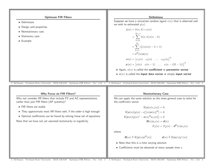
Optimum FIR Filters Definitions Suppose we have a univariate random signal x ( n ) that is observed and • Definitions we wish to estimated y ( n ) • Design and properties y ( n ) = h ( n, k ) ∗ x ( n ) ˆ • Nonstationary case M − 1 • Stationary case � = h ( n, k ) x ( n − k ) • Example k =0 M � = c ∗ k ( n ) x ( n − k + 1) k =1 = c H ( n ) x ( n ) c M ( n ) � T � c 1 ( n ) c ( n ) = c 2 ( n ) . . . � T � x ( n ) = x ( n ) x ( n − 1) x ( n − ( M − 1)) . . . • Again, c ( n ) is called the coefficient or parameter vector • x ( n ) is called the input data vector or simply input vector J. McNames Portland State University ECE 539/639 Optimum FIR Filters Ver. 1.02 1 J. McNames Portland State University ECE 539/639 Optimum FIR Filters Ver. 1.02 2 Why Focus on FIR Filters? Nonstationary Case Why not consider IIR filters that include PZ and AZ representations, We can apply the same solution as the more general case to solve for rather than just FIR filters (AP systems)? the coefficient vector • FIR filters are stable E[ x ( n ) e o ( n )] = 0 • They approximate most IIR filters well, if the order is high enough o ( n ) x ( n )] H ] = 0 E[ x ( n )[ y ( n ) − c ∗ E[ x ( n )[ y ( n ) ∗ − x ( n ) H c o ( n )]] = 0 • Optimal coefficients can be found by solving linear set of equations Note that we have not yet assumed stationarity or ergodicity R ( n ) c o ( n ) = d ( n ) P o ( n ) = P y ( n ) − d H ( n ) c o ( n ) where R ( n ) � E[ x ( n ) x H ( n )] d ( n ) � E[ x ( n ) y ∗ ( n )] • Note that this is a time varying solution • Coefficients must be obtained at every sample time n J. McNames Portland State University ECE 539/639 Optimum FIR Filters Ver. 1.02 3 J. McNames Portland State University ECE 539/639 Optimum FIR Filters Ver. 1.02 4
Comparison with Frequency-Selective Filters Performance Surface P ( c ( n )) = P y ( n ) − c H ( n ) d ( n ) − d H ( n ) c ( n ) + c H ( n ) R ( n ) c ( n ) M − 1 M � � y ( n ) = ˆ h ( n, k ) x ( n − k ) = c ∗ k ( n ) x ( n − k + 1) • Again, the error surface is a quadratic bowl k =0 k =1 • If signal is nonstationary, the bottom of the bowl changes over • Convention frequency-selective filters attenuate specified time frequency bands and amplify others • In many cases, the statistics drift slowly – These are designed given a set of specifications (e.g., stopband attenuation, passband rippled, transition bands) • Our goal then is to track the bottom of the bowl – Do not depend on data • Adaptive filters primarily solve this problem • “Optimum filters” are designed using the statistical properties of the signals (second-order moments) – Work well on all signals with those second-order moments – Note that these do not use any phase information about the input signal J. McNames Portland State University ECE 539/639 Optimum FIR Filters Ver. 1.02 5 J. McNames Portland State University ECE 539/639 Optimum FIR Filters Ver. 1.02 6 Stationary Case: Correlation Matrix Stationary Case: Cross-Correlation Vector Consider the definitions of the auto- and cross-correlation matrices � x ( n ) x ( n − M + 1) � x ( n ) = x ( n − 1) . . . � T � x ( n ) = x ( n ) x ( n − 1) x ( n − M + 1) . . . R � E[ x ( n ) x ( n ) H ] d � E[ x ( n ) y ∗ ( n )] E[ x ( n ) x ∗ ( n )] E[ x ( n ) x ∗ ( n - 1)] . . . E[ x ( n ) x ∗ ( n - M + 1)] ⎡ ⎤ ⎡ ⎤ ⎡ ⎤ r xy (0) r ∗ yx (0) ⎡ ⎤ E[ x ( n ) y ∗ ( n )] E[ x ( n - 1) x ∗ ( n )] E[ x ( n - 1) x ∗ ( n - 1)] . . . E[ x ( n - 1) x ∗ ( n - M + 1)] r xy ( − 1) yx (1) r ∗ = ⎢ ⎥ ⎢ ⎥ ⎢ ⎥ . . . E[ x ( n − 1) y ∗ ( n )] ... = ⎦ = ⎦ = . . . . . ⎣ ⎦ ⎢ ⎥ ⎢ ⎥ ⎢ ⎥ . . . . . . ⎣ ⎢ ⎥ ⎢ ⎥ . . . E[ x ( n - M + 1) x ∗ ( n )] E[ x ( n - M + 1) x ∗ ( n - 1)] . . . E[ x ( n - M + 1) x ∗ ( n - M + 1)] ⎣ ⎣ ⎦ . E[ x ( n − M + 1) y ∗ ( n )] r xy ( − M + 1) r ∗ yx ( M − 1) ⎡ ⎤ r x (0) r x (1) . . . r x ( M − 1) x (1) r x (0) r x ( M − 2) r ∗ . . . ⎢ ⎥ where we used ⎦ = R H = ⎢ . . . ⎥ ... . . . ⎢ ⎥ . . . r xy ( ℓ ) = E[ x ( n ) y ∗ ( n − ℓ )] = E[ y ( n ) x ∗ ( n + ℓ )] ∗ = r ∗ ⎣ yx ( − ℓ ) r ∗ x ( M − 1) r ∗ x ( M − 2) . . . r x (0) R becomes toeplitz J. McNames Portland State University ECE 539/639 Optimum FIR Filters Ver. 1.02 7 J. McNames Portland State University ECE 539/639 Optimum FIR Filters Ver. 1.02 8
Stationary Case Solution and Impulse Response Example 1: MA Process Create a synthetic MA process in MATLAB. Plot the pole-zero and P o = P y − d H c o Rc o = d transfer function plots of the system and the one-step ahead predictor. M − 1 Plot the MMSE versus the filter order M . For all other examples, use � c H y o ( n ) = ˆ h o ( k ) x ( n − k ) o ,n +1 = h o ( n ) M = 25 . k =0 • Draw a block diagram of the process and the estimator • The estimator and second-order statistics are no longer • What can you conclude about the relationship between the MA time-varying process and the estimator impulse response? • R becomes toeplitz, as well as Hermitian and non-negative definite • Is the estimator stable? • Optimum filter is time-invariant • Why can’t we make the MSE → 0 as M → ∞ ? • On average (across realizations) performs better than any other linear filter of the same order J. McNames Portland State University ECE 539/639 Optimum FIR Filters Ver. 1.02 9 J. McNames Portland State University ECE 539/639 Optimum FIR Filters Ver. 1.02 10 Example 1: Work Space Example 1: Pole Zero Plots AZ System Estimator 1 1 0.5 0.5 0 0 −0.5 −0.5 −1 −1 −1 −0.5 0 0.5 1 −1 −0.5 0 0.5 1 J. McNames Portland State University ECE 539/639 Optimum FIR Filters Ver. 1.02 11 J. McNames Portland State University ECE 539/639 Optimum FIR Filters Ver. 1.02 12
Example 1: Impulse Responses Example 1: Transfer Functions 1 3 Impulse Response | H ( e jω ) | 2 0 1 0 −1 0 0.1 0.2 0.3 0.4 0.5 0.6 0.7 0.8 0.9 1 0 5 10 15 20 25 Frequency (normalized) Lag (samples) 1 Impulse Response 3 | H ( e jω ) | 2 0 1 0 −1 0 0.1 0.2 0.3 0.4 0.5 0.6 0.7 0.8 0.9 1 0 5 10 15 20 25 Frequency (normalized) Lag (samples) J. McNames Portland State University ECE 539/639 Optimum FIR Filters Ver. 1.02 13 J. McNames Portland State University ECE 539/639 Optimum FIR Filters Ver. 1.02 14 Example 1: Predicted Segment Example 1: MMSE Versus Filter Order 2.5 5 Actual 4 Predicted 2 3 2 Output (scaled) 1.5 MMSE 1 0 1 −1 −2 0.5 −3 0 −4 0 20 40 60 80 100 0 10 20 30 40 50 60 70 80 90 100 Filter Order Time (Samples J. McNames Portland State University ECE 539/639 Optimum FIR Filters Ver. 1.02 15 J. McNames Portland State University ECE 539/639 Optimum FIR Filters Ver. 1.02 16
Recommend
More recommend
Explore More Topics
Stay informed with curated content and fresh updates.
