Optimization and Simulation Statistical analysis and bootstrapping - - PowerPoint PPT Presentation

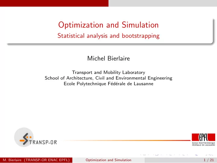
Optimization and Simulation

Statistical analysis and bootstrapping Michel Bierlaire

Transport and Mobility Laboratory School of Architecture, Civil and Environmental Engineering Ecole Polytechnique F´ ed´ erale de Lausanne

• M. Bierlaire (TRANSP-OR ENAC EPFL)

Optimization and Simulation 1 / 21

Introduction

The outputs of the simulator are random variables. Running the simulator provides one realization of these r.v. We have no access to the pdf or CDF of these r.v. Well... this is actually why we rely on simulation. How to derive statistics about a r.v. when only instances are known? How to measure the quality of this statistic?

• M. Bierlaire (TRANSP-OR ENAC EPFL)

Optimization and Simulation 2 / 21

Sample mean and variance

Consider X1, . . . , Xn i.i.d. r.v. E[Xi] = µ, Var(Xi) = σ2. The sample mean ¯ X = 1 n

n

• i=1

Xi is an unbiased estimate of the population mean µ, as E[ ¯ X] = µ. The sample variance S2 = 1 n − 1

n

• i=1

(Xi − ¯ X)2 is an unbiased estimator of the population variance σ2, as E[S2] = σ2. (see proof: Ross, chapter 7)

• M. Bierlaire (TRANSP-OR ENAC EPFL)

Optimization and Simulation 3 / 21

Sample mean and variance

Recursive computation

1 Initialize ¯

X0 = 0, S2

1 = 0.

2 Update the mean

¯ Xk+1 = ¯ Xk + Xk+1 − ¯ Xk k + 1

3 Update the variance

S2

k+1 =

• 1 − 1

k

• S2

k + (k + 1)( ¯

Xk+1 − ¯ Xk)2.

• M. Bierlaire (TRANSP-OR ENAC EPFL)

Optimization and Simulation 4 / 21

Mean Square Error

Consider X1, . . . , Xn i.i.d. r.v. with CDF F. Consider a parameter θ(F) of the distribution (mean, quantile, mode, etc.) Consider θ(X1, . . . , Xn) an estimator of θ(F). The Mean Square Error of the estimator is defined as MSE(F) = EF

• θ(X1, . . . , Xn) − θ(F)

2 , where EF emphasizes that the expectation is taken under the assumption that the r.v. all have distribution F. If F is unknown, it is not immediate to find an estimator of MSE.

• M. Bierlaire (TRANSP-OR ENAC EPFL)

Optimization and Simulation 5 / 21

How many draws must be used?

Let X a r.v. with mean θ and variance σ2. We want to estimate the mean θ of the simulated distribution. The estimator used is the sample mean: ¯ X. The mean square error is E[( ¯ X − θ)2] = σ2 n The sample mean ¯ X is normally distributed with mean θ and variance σ2/n. So we can stop generating data when σ/√n is small. σ is approximated by the sample variance S. Law of large numbers: at least 100 draws (say) should be used. See Ross p. 121 for details.

• M. Bierlaire (TRANSP-OR ENAC EPFL)

Optimization and Simulation 6 / 21

Mean Square Error

Other indicators than the mean are desired. Theoretical results about the MSE cannot always be derived. Solution: rely on simulation. Method: bootstrapping.

• M. Bierlaire (TRANSP-OR ENAC EPFL)

Optimization and Simulation 7 / 21

Empirical distribution function

Consider X1, . . . , Xn i.i.d. r.v. with CDF F. Consider a realization x1,. . . ,xn of these r.v. The empirical distribution function is defined as Fe(x) = 1 n

n

• i=1

I{xi ≤ x}, where I{xi ≤ x} = 1 if xi ≤ x,

• therwise.

CDF of a r.v. that can take any xi with equal probability.

• M. Bierlaire (TRANSP-OR ENAC EPFL)

Optimization and Simulation 8 / 21

Empirical CDF

0.1 0.2 0.3 0.4 0.5 0.6 0.7 0.8 0.9 1 0.5 1 1.5 2 2.5 3 3.5 4 Fe(x), n = 10 F(x)

• M. Bierlaire (TRANSP-OR ENAC EPFL)

Optimization and Simulation 9 / 21

Empirical CDF

0.1 0.2 0.3 0.4 0.5 0.6 0.7 0.8 0.9 1 1 2 3 4 5 6 7 8 Fe(x), n = 100 F(x)

• M. Bierlaire (TRANSP-OR ENAC EPFL)

Optimization and Simulation 10 / 21

Empirical CDF

0.1 0.2 0.3 0.4 0.5 0.6 0.7 0.8 0.9 1 1 2 3 4 5 6 7 8 Fe(x), n = 1000 F(x)

• M. Bierlaire (TRANSP-OR ENAC EPFL)

Optimization and Simulation 11 / 21

From reality to data

Reality Data Random variable X Xe CDF F Fe True parameter θ(F) θ(Fe) Sample X1, . . . , Xn ∼ F X e

1 , . . . , X e n ∼ Fe

Estimate

• θ(X1, . . . , Xn)
• θ(X e

1 , . . . , X e n )

• M. Bierlaire (TRANSP-OR ENAC EPFL)

Optimization and Simulation 12 / 21

Mean Square Error

We use the empirical distribution function Fe We can approximate MSE(F) = EF

• θ(X1, . . . , Xn) − θ(F)

2 , by MSE(Fe) = EFe

• θ(X e

1 , . . . , X e n ) − θ(Fe)

2 , θ(Fe) can be computed directly from the data (mean, variance, etc.)

• M. Bierlaire (TRANSP-OR ENAC EPFL)

Optimization and Simulation 13 / 21

Mean Square Error

We want to compute MSE(Fe) = EFe

• θ(X e

1 , . . . , X e n ) − θ(Fe)

2 , X e

i are r.v. that can take any xi with equal probability.

Therefore, MSE(Fe) = 1 nn

n

• i1=1

· · ·

n

• in=1
• θ(xi1, . . . , xin) − θ(Fe)

2 , Clearly impossible to compute when n is large. Solution: simulation.

• M. Bierlaire (TRANSP-OR ENAC EPFL)

Optimization and Simulation 14 / 21

Bootstrapping

For r = 1, . . . , R Draw xr

1,. . . ,xr n from Fe, that is draw from the data:

1

Let s be a draw from U[0, 1]

2

Set j = floor(ns).

3

Return xj.

Compute Mr =

• θ(xr

1, . . . , xr n) − θ(Fe)

2 , Estimate of MSE(Fe) and, therefore, of MSE(F): 1 R

R

• r=1

Mr Typical value for R: 100.

• M. Bierlaire (TRANSP-OR ENAC EPFL)

Optimization and Simulation 15 / 21

Bootstrap: simple example

Data: 0.636, -0.643, 0.183, -1.67, 0.462 Mean= -0.206 MSE= E[( ¯ X − θ)2] = S2/n= 0.1817

r ˆ θ θ(Fe) MSE 1

• 0.643
• 0.643
• 0.643

0.462 0.462

• 0.201
• 0.206

2.544e-05 2

• 0.643

0.183 0.636 0.636 0.636 0.2896

• 0.206

0.2456 3

• 1.67
• 1.67

0.183 0.462 0.636

• 0.411
• 0.206

0.04204 4

• 1.67
• 0.643

0.183 0.183 0.636

• 0.2617
• 0.206

0.003105 5

• 0.643

0.462 0.462 0.636 0.636 0.3105

• 0.206

0.2667 6

• 1.67
• 1.67

0.183 0.183 0.183

• 0.5573
• 0.206

0.1234 7

• 0.643

0.183 0.183 0.462 0.636 0.1642

• 0.206

0.137 8

• 1.67
• 1.67
• 0.643

0.183 0.183

• 0.7225
• 0.206

0.2667 9 0.183 0.462 0.462 0.636 0.636 0.4756

• 0.206

0.4646 10

• 0.643

0.183 0.183 0.462 0.636 0.1642

• 0.206

0.137 0.1686

• M. Bierlaire (TRANSP-OR ENAC EPFL)

Optimization and Simulation 16 / 21

Python code

def bootstrap(data): n = len(data) b = [] for i in range(0,n): r = random() index = int(n*r) b.append(data[index]) return b def percentile(dataSorted,p): i = max(int(round(p * len(dataSorted) + 0.5)), 2) return dataSorted[i-2]

• M. Bierlaire (TRANSP-OR ENAC EPFL)

Optimization and Simulation 17 / 21

95% percentile: Python code

N = 10000 data = drawNormal(N) data.sort() theP = 0.975 quantile = float(percentile(data,theP)) print("{}% quantile={:.4f}".format(theP,quantile)) R=100 sum = 0.0 for l in range (0,R): b = bootstrap(data) b.sort() q = float(percentile(b,theP)) sum += (quantile-q)**2 print("MSE: {:.4f} sqrt(MSE): {:.4f}".format(sum/R,sqrt(sum/(R

• M. Bierlaire (TRANSP-OR ENAC EPFL)

Optimization and Simulation 18 / 21

Results

N=10000 0.975% quantile=1.9472 MSE: 0.0009 sqrt(MSE): 0.0303 N=1000 0.975% quantile=1.8808 MSE: 0.0098 sqrt(MSE): 0.0988 N=100 0.975% quantile=1.4078 MSE: 0.0300 sqrt(MSE): 0.1732

• M. Bierlaire (TRANSP-OR ENAC EPFL)

Optimization and Simulation 19 / 21

Summary

The number of draws is determined by the required precision. In some cases, the precision is derived from theoretical results. If not, rely on bootstrapping. Idea: use simulation to estimate the Mean Square Error.

• M. Bierlaire (TRANSP-OR ENAC EPFL)

Optimization and Simulation 20 / 21

Appendix: MSE for the mean

Consider X1, . . . , Xn i.i.d. r.v. Denote θ = E[Xi] and σ2 = Var(Xi). Consider ¯ X = n

i=1 Xi/n.

E[ ¯ X] = n

i=1 E[Xi]/n = θ.

MSE: E[( ¯ X − θ)2] = Var ¯ X = Var n

• i=1

Xi/n

• =

n

• i=1

Var(Xi)/n2 = σ2/n.

• M. Bierlaire (TRANSP-OR ENAC EPFL)

Optimization and Simulation 21 / 21