Optimization and Simulation Constrained optimization Michel - PowerPoint PPT Presentation
Optimization and Simulation Constrained optimization Michel Bierlaire michel.bierlaire@epfl.ch Transport and Mobility Laboratory Optimization and Simulation p. 1/51 The problem Generic problem: x R n f ( x ) min subject to [ h : R n
Optimization and Simulation Constrained optimization Michel Bierlaire michel.bierlaire@epfl.ch Transport and Mobility Laboratory Optimization and Simulation – p. 1/51
The problem Generic problem: x ∈ R n f ( x ) min subject to [ h : R n → R m ] h ( x ) = 0 [ g : R n → R p ] g ( x ) ≤ 0 ⊆ R n x ∈ X Optimization and Simulation – p. 2/51
Outline • Feasible directions, constraint qualification • Optimality conditions • Convex constraints • Lagrange multipliers: necessary conditions • Lagrange multipliers: sufficient conditions • Algorithms • Constrained Newton • Interior point • Augmented lagrangian • Sequential quadratic programming Optimization and Simulation – p. 3/51
Feasible directions Definitions: • x ∈ R n is a feasible point if it verifies the constraints • Given x feasible, d is a feasible direction in x if there is η > 0 such that x + αd is feasible for any 0 ≤ α ≤ η . Convex constraints: • Let X ⊆ R n be a convex set, and x , y ∈ X , x � = y . • The direction d = y − x is feasible in x . • Moreover, for each 0 ≤ α ≤ 1 , αx + (1 − α ) y is feasible. Optimization and Simulation – p. 4/51
Feasible directions Corollary: • Let X ⊆ R n • Let x be an interior point, that is there exists ε > 0 such that � x − z � ≤ ε = ⇒ z ∈ X. • Then, any direction d is feasible in x . Optimization and Simulation – p. 5/51
Feasible sequences • Consider the generic optimization problem • Let x + ∈ R n be a feasible point • The sequence ( x k ) k is said to be feasible in x + if • lim k →∞ x k = x + , • ∃ k 0 such that x k is feasible if k ≥ k 0 , • x k � = x + for all k . Optimization and Simulation – p. 6/51
Feasible sequence: example • One equality constraint h ( x ) = x 2 1 − x 2 = 0 , • Feasible point: x + = (0 , 0) T • Feasible sequence: � � 1 k x k = 1 k 2 Optimization and Simulation – p. 7/51
Feasible sequence: example • h ( x ) = x 2 1 − x 2 = 0 x 2 • • • • • • • • • • • • • • • • • • • x + = 0 -1 -0.5 0 0.5 1 x 1 Optimization and Simulation – p. 8/51
Feasible limiting direction Idea: consider the sequence of directions x k − x + d k = � x k − x + � , and take the limit. • Directions d k are not necessarily feasible • The sequence may not always converge • Subsequences must then be considered Optimization and Simulation – p. 9/51
Feasible limiting direction: example • d 1 h ( x ) = x 2 1 − x 2 = 0 x 2 d 2 d 3 • • • d • • • • • • • • • • • • • • • • x + = 0 -1 -0.5 0 0.5 1 x 1 Optimization and Simulation – p. 10/51
Feasible limiting direction: example • Constraint: h ( x ) = x 2 1 − x 2 = 0 • Feasible point: x + = (0 , 0) T • Feasible sequence: � ( − 1) k � x k = k 1 k 2 • Sequence of directions: ( − 1) k k � � √ k 2 +1 d k = 1 k 2 +1 , √ • Two limiting directions Optimization and Simulation – p. 11/51
Feasible limiting direction: example h ( x ) = x 2 • 1 − x 2 = 0 d 1 x 2 d 2 d 3 d 4 • • • d ′′ d ′ • • • • • • • • • • • • • • • x + = 0 -1 -0.5 0 0.5 1 x 1 Optimization and Simulation – p. 12/51
Feasible limiting direction • Consider the generic optimization problem • Let x + ∈ R n be feasible • Let ( x k ) k be a feasible sequence in x + • Then, d � = 0 is a feasible limiting direction in x + for the sequence ( x k ) k if there exists a subsequence ( x k i ) i such that x k i − x + d � d � = lim � x k i − x + � . i →∞ Notes: • It is sometimes called a tangent direction. • Any feasible direction d is also a limiting feasible direction, for the sequence x k = x + + 1 k d Optimization and Simulation – p. 13/51
Cone of directions • Consider the generic optimization problem • Let x + ∈ R n be feasible • The set of directions d such that d T ∇ g i ( x + ) ≤ 0 , ∀ i = 1 , . . . , p such that g i ( x + ) = 0 , and d T ∇ h i ( x + ) = 0 , i = 1 , . . . , m, as well as their multiples αd , α > 0 , is the cone of directions at x + . Optimization and Simulation – p. 14/51
Cone of directions h ( x ) = x 2 1 − x 2 = 0 x 2 d ′′ d ′ x + = 0 ∇ h ( x + ) -1 -0.5 0 0.5 1 x 1 Optimization and Simulation – p. 15/51
Cone of directions Theorem: • Consider the generic optimization problem • Let x + ∈ R n be feasible • If d is a limiting feasible direction at x + • Then d belongs to the cone of directions at x + Optimization and Simulation – p. 16/51
Constraint qualification Definition: • Consider the generic optimization problem • Let x + ∈ R n be feasible • The constraint qualification condition is verified if every direction in the cone of directions at x + is a feasible limiting direction at x + . This is verified in particular • if the constraints are linear, or • if the gradients of the constraints active at x + are linearly independent. Optimization and Simulation – p. 17/51
Optimality conditions Necessary condition for the generic problem: • Let x ∗ be a local minimum of the generic problem • Then ∇ f ( x ∗ ) T d ≥ 0 for each direction d which is feasible limiting at x ∗ . Intuition: no “feasible” direction is a descent direction Optimization and Simulation – p. 18/51
Optimality conditions: convex problem (I) Consider the problem min x f ( x ) subject to x ∈ X ⊆ R n where X is convex and not empty. • If x ∗ is a local minimum of this problem • Then, for any x ∈ X , ∇ f ( x ∗ ) T ( x − x ∗ ) ≥ 0 . Optimization and Simulation – p. 19/51
Optimality conditions: convex problem (II) • Assume now that X is convex and closed. • For any y ∈ R n , we note by [ y ] P the projection of y on X . • If x ∗ is a local minimum, then x ∗ = [ x ∗ − α ∇ f ( x ∗ )] P ∀ α > 0 . • Moreover, if f is convex, the condition is sufficient. Note: useful when the projection is easy to compute (e.g. bound constraints) Optimization and Simulation – p. 20/51
Optimality conditions: Karush-Kuhn-Tucker The problem: x ∈ R n f ( x ) min subject to [ h : R n → R m ] h ( x ) = 0 [ g : R n → R p ] g ( x ) ≤ 0 = R n x ∈ X • Let x ∗ be a local minimum • Let L be the Lagrangian L ( x, λ, µ ) = f ( x ) + λ T h ( x ) + µ T g ( x ) . • Assume that the constraint qualification condition is verified. • Then... Optimization and Simulation – p. 21/51
Optimality conditions: Karush-Kuhn-Tucker ... there exists a unique λ ∗ ∈ R m and a unique µ ∗ ∈ R p such that ∇ x L ( x ∗ , λ ∗ , µ ∗ ) = ∇ f ( x ∗ ) + ( λ ∗ ) T ∇ h ( x ∗ ) + ( µ ∗ ) T ∇ g ( x ∗ ) = 0 , µ ∗ j ≥ 0 j = 1 , . . . , p, and µ ∗ j g j ( x ∗ ) = 0 j = 1 , . . . , p. If f , g and h are twice differentiable, we also have y T ∇ 2 xx L ( x ∗ , λ ∗ , µ ∗ ) y ≥ 0 ∀ y � = 0 such that y T ∇ h i ( x ∗ ) = 0 i = 1 , . . . , m y T ∇ g i ( x ∗ ) = 0 i = 1 , . . . , p such that g i ( x ∗ ) = 0 . Optimization and Simulation – p. 22/51
KKT: sufficient conditions Let x ∗ ∈ R n , λ ∗ ∈ R m and µ ∗ ∈ R p be such that ∇ x L ( x ∗ , λ ∗ , µ ∗ ) = 0 h ( x ∗ ) = 0 , g ( x ∗ ) ≤ 0 µ ∗ ≥ 0 , µ ∗ j g j ( x ∗ ) = 0 µ ∗ ∀ j such that g i ( x ∗ ) = 0 . ∀ j, j > 0 y T ∇ 2 xx L ( x ∗ , λ ∗ , µ ∗ ) y > 0 ∀ y � = 0 such that y T ∇ h i ( x ∗ ) = 0 i = 1 , . . . , m y T ∇ g i ( x ∗ ) = 0 i = 1 , . . . , p such that g i ( x ∗ ) = 0 . Then x ∗ is a strict local minimum of the problem. Optimization and Simulation – p. 23/51
Algorithms • Constrained Newton • Interior point • Augmented lagrangian • Sequential quadratic programming Here: we give the main ideas. Optimization and Simulation – p. 24/51
Constrained Newton Context: • Problem with a convex constraint set. • Assumption: it is easy to project on the set. • Examples: bound constraints, linear constraints. Main idea: • In the unconstrained case, Newton = preconditioned steepest descent • Consider first the projected gradient method • Precondition it. Optimization and Simulation – p. 25/51
Projected gradient method 3 2.5 2 1.5 x 2 1 x 0 0.5 0 x ∗ -0.5 0.5 1 1.5 2 2.5 3 3.5 4 4.5 5 x 1 Optimization and Simulation – p. 26/51
Condition number • Consider ∇ 2 f ( x ) positive definite. • Let λ 1 be the largest eigenvalue, and λ n the smallest. • The condition number is equal to λ 1 /λ n . • Geometrically, it is the ratio between the largest and the smallest curvature. • The closest it is to one, the better. Optimization and Simulation – p. 27/51
Condition number 2 2 1 1 0 x 2 0 x 2 -1 -1 -2 -2 -2 -1 0 1 2 -2 -1 0 1 2 x 1 x 1 Cond = 9/2 Cond = 1 Optimization and Simulation – p. 28/51
Recommend
More recommend
Explore More Topics
Stay informed with curated content and fresh updates.
