Optimal Randomized Algorithms for Integration Integration on - PowerPoint PPT Presentation

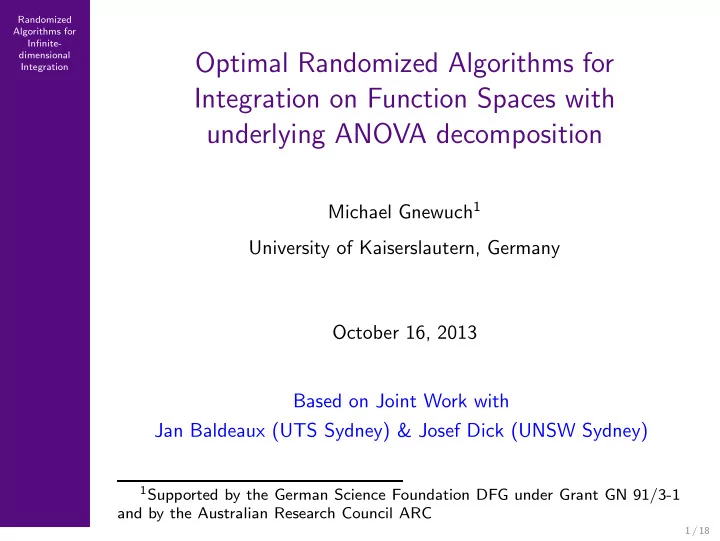
Randomized Algorithms for Infinite- dimensional Optimal Randomized Algorithms for Integration Integration on Function Spaces with underlying ANOVA decomposition Michael Gnewuch 1 University of Kaiserslautern, Germany October 16, 2013 Based on Joint Work with Jan Baldeaux (UTS Sydney) & Josef Dick (UNSW Sydney) 1 Supported by the German Science Foundation DFG under Grant GN 91/3-1 and by the Australian Research Council ARC 1 / 18

Randomized ANOVA Decomposition ( ∞ -Variate Functions) Algorithms for Infinite- dimensional Integration Sequence space [0 , 1] N , endowed with probability measure d x = ⊗ j ∈ N d x j . For f ∈ L 2 ([0 , 1] N ) , u ⊂ f N : � f ∅ ( x ) := [0 , 1] N f ( y ) d y , � � f u ( x ) := [0 , 1] [ N ] \ u f ( x u , y N \ u ) d y N \ u − f v ( x ) , v � u where x u = ( x j ) j ∈ u , y N \ u = ( y j ) j ∈ N \ u . Then � 1 f u ( x ) d x j = 0 for j ∈ u . 0 This implies � � in L 2 ([0 , 1] N ) , f = f u and Var( f ) = Var( f u ) . u ⊂ f N u ⊂ f N 2 / 18

Randomized Algorithms for Function Spaces of Integrands Infinite- dimensional Integration Construction of spaces of integrands f : [0 , 1] N → R : • Reproducing kernel Hilbert space H = H ( k ) of univariate � 1 functions f : [0 , 1] → R with 0 f ( x ) d x = 0 . • Hilbert spaces H u of multivariate functions f u : [0 , 1] u �→ R : H u := � ⊗ j ∈ u H for u ⊂ f N , H ∅ = span { 1 } . where • Hilbert space H γ of functions of infinitely many variables: Weights γ = ( γ u ) u ⊂ f N with � u ⊂ f N γ u < ∞ � � � � � � � � f u ∈ H u , � f � 2 γ − 1 u � f u � 2 H γ := H u < ∞ f u H γ := , u ⊂ f N u ⊂ f N where H γ ⊂ L 2 ([0 , 1] N ) and f = � u ⊂ f N f u ANOVA decomposition. 3 / 18

Randomized Weights Algorithms for Infinite- dimensional Integration Product weights γ [Sloan & Wo´ zniakowski’98]: Let γ 1 ≥ γ 2 ≥ γ 3 ≥ · · · ≥ 0 . Then γ u := � j ∈ u γ j . Finite-order weights γ of order ω [Dick, Sloan, Wang & Wo´ zniakowski’06]: γ u = 0 for all | u | > ω . Finite-intersection weights γ of degree ρ : Finite-order weights with |{ u ⊂ f N | γ u > 0 , u ∩ v � = ∅}| ≤ 1 + ρ for all v ⊂ f N , γ v > 0 . (Subclass of finite-intersection weights are the “finite-diameter weights” proposed by Creutzig.) � � � � � � γ 1 /p decay := sup p ∈ R < ∞ . � u � u ⊂ f N 4 / 18

Integration, Algorithms & Cost Model Randomized Algorithms for Infinite- � dimensional Integration Integration functional I on H γ : I ( f ) := [0 , 1] N f ( x ) d x Admissable randomized algorithms: n � α i f ( t ( i ) where t ( i ) v i ∈ [0 , 1] v i , v i ⊂ f N , a = 1 / 2 Q n ( f ) = v i ; a ) , i =1 Nested Subspace Sampling [Creutzig, Dereich, M¨ uller-Gronbach, Ritter‘09]: Fix s ≥ 1 . n � � � s cost nest ( Q n ) := max v i i =1 Unrestricted Subspace Sampling [Kuo, Sloan, Wasilkowski, Wo´ zniakowski‘10]: Fix s ≥ 1 . n � | v i | s cost unr ( Q n ) := i =1 5 / 18

Randomized Algorithms for Infinite- Randomized Setting dimensional Integration Error criterion: (worst case) randomized error � ( I ( f ) − Q ( f )) 2 � e ran ( Q ; H γ ) 2 := sup E � f � H γ ≤ 1 N th minimal randomized error: mod ∈ { nest , unr } , e ran mod ( N ) := inf { e ran ( Q ; H γ ) | Q adm. rand. alg. , cost mod ( Q ) ≤ N } . “Convergence order” of e ran mod ( N ) : � � mod ( N ) · N t < ∞ λ ran e ran mod := sup t > 0 | sup . N ∈ N 6 / 18

Nested Subspace Sampling: Multilevel Algorithms Randomized Algorithms for Infinite- dimensional For levels k = 1 , . . . , m : v k := { 1 , . . . , 2 k } . n 1 ≥ n 2 ≥ n 3 ≥ · · · . Integration (Unbiased) RQMC Algorithms: n k � Q v k ( g ) := 1 g ( t ( j,k ) t ( j,k ) ∈ [0 , 1] v k . ) , v k v k n k j =1 Projections: Ψ v k f ( x ) := f ( x v k ; a ) for k ≥ 1 and Ψ v 0 f ( x ) := 0 . RQMC-Multilevel Algorithm: m � Q ML m ( f ) := Q v k (Ψ v k f − Ψ v k − 1 f ) . k =1 m � cost nest ( Q ML m ) = cost unr ( Q ML 2 n k 2 ks . Cost: m ) ≤ k =1 7 / 18

Nested Subspace Sampling: Multilevel Algorithms Randomized Algorithms for Infinite- dimensional Integration Projections: Ψ v k f ( x ) = f ( x v k ; a ) for k ≥ 1 and Ψ v 0 f ( x ) = 0 . m � Q ML RQMC-ML Algo.: m ( f ) = Q v k (Ψ v k f − Ψ v k − 1 f ) . k =1 Then m � � � Q ML m ( f ) = I (Ψ v k f − Ψ v k − 1 f ) = I (Ψ v m f ) , E k =1 and �� � 2 � I ( f ) − Q ML m ( f ) E m � � � = | I ( f ) − I (Ψ v m f ) | 2 + Var Q v k (Ψ v k f − Ψ v k − 1 f ) . k =1 8 / 18

Randomized Algorithms for Infinite- dimensional Integration Multilevel Algorithms Multilevel Monte Carlo algorithms were introduced in the context of integral equations and parametric integration by Heinrich (1998) and Heinrich and Sindambiwe (1999) and in the context of stochastic differential equations by Giles (2008). Multilevel quasi-Monte Carlo algorithms were tested by Giles and Waterhouse (2009). Multilevel Monte Carlo and quasi-Monte Carlo algorithms have been studied in a number of papers, see, e.g., the web page of Mike Giles http://people.maths.ox.ac.uk/gilesm/mlmc community.html for more recent information. 9 / 18

Randomized Algorithms for Nested Subspace Sampling Infinite- dimensional Integration Unanchored reproducing kernel k of H : For x, y ∈ [0 , 1] : 3 + x 2 + y 2 k ( x, y ) = 1 − max { x, y } 2 H = H ( k ) consists of functions f ∈ L 2 ([0 , 1]) with f absolutely � 1 continuous, f (1) ∈ L 2 ([0 , 1]) , and 0 f ( x ) d x = 0 . k induces ANOVA decomposition on H γ : � 1 � f = f u , f u ∈ H u , and f u ( x ) d x j = 0 if j ∈ u . 0 u ⊂ f N 10 / 18

Randomized Nested Subspace Sampling: Product Weights Algorithms for Infinite- dimensional Theorem [Baldeaux, G.‘12]. γ product weights, decay > 1 . Then Integration λ ran decay ≥ 1 + 3 s : nest = 3 / 2 nest = decay − 1 λ ran 1 + 3 s ≥ decay > 1 : 2 s (Upper error bound via multilevel algorithms based on scrambled polynomial lattice rules (scrambling: Owen‘95; polynomial lattice rules: Niederreiter‘92); lower error bound holds for general randomized algorithms.) Comparison with previously known results for s = 1 : [Hickernell, Niu, M¨ uller-Gronbach, Ritter‘10]: Multilevel algorithms ˜ Q ML based on scrambled Niederreiter ( t, m, s ) -nets: m decay ≥ 11 : λ ran nest = 3 / 2 [Baldeaux‘11]: Multilevel algorithms ˆ Q ML based on scrambled m polynomial lattice rules: decay ≥ 10 : λ ran nest = 3 / 2 11 / 18

Randomized Algorithms for Infinite- dimensional Integration Nested Subspace Sampling: Finite-Intersection Weights Theorem [Baldeaux, G.‘12]. γ be finite-intersection weights, decay > 1 . Then λ ran decay ≥ 1 + 3 s : nest = 3 / 2 nest = decay − 1 λ ran 1 + 3 s ≥ decay > 1 : 2 s (Upper error bound achieved by multilevel algorithms based on scrambled polynomial lattice rules; lower error bound holds for general randomized algorithms.) 12 / 18

Randomized Algorithms for Unrestricted Subspace Sampling: CDAs (alias MDMs) Infinite- dimensional Integration Anchored decomposition: � f ∅ , a := f ( a ) and f u, a ( x ) := f ( x u ; a ) − f v, a ( x ) . v � u A changing dimension algorithm (or multivariate decomposition method) Q CD is of the form � Q CD ( f ) = Q u,n u ( f u, a ) , u ⊂ f N � Q u,n u using n u samples to approximate [0 , 1] u f u, a ( x u ) d x u . Q CD is linear if Q u,n u s are linear: f u, a ( x ) = � v ⊆ u ( − 1) | u \ v | f ( x v ; a ) [Kuo, Sloan, Wasilkowski, Wo´ zniakowski’10a] Cost for evaluating f u, a in unrestricted model: O (2 | u | | u | s ) . 13 / 18

Randomized Algorithms for Infinite- dimensional Integration Changing Dimension Algorithms Changing dimension algorithms (alias “multivariate decomposition methods”) for infinite-dimensional integration were introduced in [Kuo, Sloan, Wasilkowski, Wo´ zniakowski’10] and refined in [Plaskota & Wasilkowski’11]. These algorithms have also been adapted to infinite-dimensional approximation problems, see the papers of Wasilkowski and of Wasilkowski & Wo´ zniakowski. A similar idea was used for multivariate integration in [Griebel & Holtz’10] (“dimension-wise quadrature methods”). 14 / 18

Randomized Algorithms for Unrestricted Subspace Sampling Infinite- dimensional Integration Unanchored reproducing kernel k χ of smoothness χ : x, y ∈ [0 , 1] χ � B τ ( x ) B τ ( y ) + ( − 1) χ +1 B 2 χ ( | x − y | ) k χ ( x, y ) = , τ ! τ ! (2 χ )! τ =1 where B τ is Bernoulli polynomial of degree τ . H = H ( k χ ) consists of functions f ∈ L 2 ([0 , 1]) with f, f (1) , . . . , f ( χ − 1) absolutely continuous, f ( χ ) ∈ L 2 ([0 , 1]) , and � 1 0 f ( x ) d x = 0 . k χ induces ANOVA decomposition on H γ : � 1 � f = f u , f u ∈ H u , and f u ( x ) d x j = 0 if j ∈ u . 0 u ⊂ f N 15 / 18