QMC methods for stochastic programs: Contents ANOVA decomposition - PowerPoint PPT Presentation

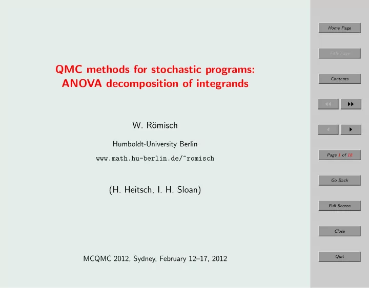
Home Page Title Page QMC methods for stochastic programs: Contents ANOVA decomposition of integrands ◭◭ ◮◮ W. R¨ omisch ◭ ◮ Humboldt-University Berlin Page 1 of 18 www.math.hu-berlin.de/~romisch Go Back (H. Heitsch, I. H. Sloan) Full Screen Close Quit MCQMC 2012, Sydney, February 12–17, 2012

Introduction Home Page • Stochastic programs are optimization problems containing in- tegrals in the objective function and/or constraints. Title Page • Applied stochastic programming models in production, trans- Contents portation, energy, finance etc. are typically large scale. ◭◭ ◮◮ • Standard approach for solving such models are variants of Monte Carlo for generating scenarios (i.e., samples). ◭ ◮ • A few recent approaches to scenario generation in stochastic Page 2 of 18 programming besides MC: (a) Optimal quantization of probability distributions (Pflug-Pichler Go Back 2010) . Full Screen (b) Quasi-Monte Carlo (QMC) methods (Koivu-Pennanen 05, Homem- de-Mello 06) . Close (c) Sparse grid quadrature rules (Chen-Mehrotra 08) . Quit

Home Page While the justification of MC and (a) may be based on available sta- Title Page bility results for stochastic programs, there is almost no reasonable justification of applying (b) and (c). Contents Personal interest: Applying and justifying randomized QMC ◭◭ ◮◮ methods (randomly shifted and digitally shifted polynomial lattice ◭ ◮ rules) with application in energy models. Page 3 of 18 Go Back Full Screen Close Quit

Two-stage linear stochastic programs Home Page Two-stage stochastic programs arise as deterministic equivalents of improperly posed random linear programs Title Page min {� c, x � : x ∈ X, Tx = ξ } , Contents where X is a convex polyhedral subset of R m , T a matrix, ξ is a ◭◭ ◮◮ d -dimensional random vector. A possible deviation ξ − Tx is compensated by additional costs ◭ ◮ Φ( x, ξ ) whose mean with respect to the probability distribution P of ξ is added to the objective. We assume that the additional costs Page 4 of 18 represent the optimal value of a second-stage program , namely, Go Back Φ( x, ξ ) = inf {� q, y � : y ∈ R ¯ m , Wy = ξ − Tx, y ≥ 0 } , where q ∈ R ¯ m , W a ( d, ¯ m ) -matrix (having rank d ) and t varies in Full Screen the polyhedral cone W ( R ¯ m + ) . The deterministic equivalent then is of the form Close � � � � c, x � + R d Φ( x, ξ ) P ( dξ ) : x ∈ X min . Quit

We assume that the additional costs are of the form Home Page Φ( x, ξ ) = ϕ ( ξ − Tx ) with the second-stage optimal value function Title Page Contents ϕ ( t ) = inf {� q, y � : Wy = t, y ≥ 0 } = sup {� t, z � : W ⊤ z ≤ q } = sup � t, z � , ◭◭ ◮◮ z ∈D ◭ ◮ There exist vertices v j of the dual feasible set D and polyhedral cones K j , j = 1 , . . . , ℓ , decomposing dom ϕ such that Page 5 of 18 ϕ ( t ) = � v j , t � , ∀ t ∈ K j , j =1 ,...,ℓ � v j , t � . and ϕ ( t ) = max Go Back Hence, the integrands are of the form Full Screen j =1 ,...,ℓ � v j , ξ − Tx � . f ( ξ ) = max Close Problem: When transformed to [0 , 1] d , f is not of bounded variation in the Hardy-Krause sense and does not belong to tensor product Quit Sobolev spaces � d i =1 W 1 2 ([0 , 1]) in general.

Model extensions Home Page • Two-stage models with affine functions h ( ξ ) and/or T ( ξ ) , hence, the integrands f are of the form Title Page j =1 ,...,ℓ � v j , h ( ξ ) − T ( ξ ) x � . f ( ξ ) = max Contents • Two-stage models with random second-stage costs q ( ξ ) ◭◭ ◮◮ j =1 ,...,ℓ � v j ( ξ ) , h ( ξ ) − Tx � = max j =1 ,...,ℓ � C j q ( ξ ) , h ( ξ ) − T ( ξ ) x � . f ( ξ )= max ◭ ◮ • Multi-period models : Random vector ξ = ( ξ 1 , . . . , ξ T ) f ( ξ ) = Ψ 1 ( ξ, x ) , Page 6 of 18 where Ψ 1 is given by the DP recursion Go Back � u t − 1 , z t � + Ψ t +1 ( ξ t , z t ) : W ⊤ Φ t ( ξ t , u t − 1 ) := sup � � t z t ≤ q t ( ξ t ) Ψ t ( ξ t , z t − 1 ) := Φ t ( ξ t , h t ( ξ t ) − T t ( ξ t ) z t − 1 ) , t = T, . . . , 1 , Full Screen where z 0 = x , ξ t = ( ξ t , . . . , ξ T ) and Ψ T +1 ( ξ T +1 , z T ) ≡ 0 . Close • Multi-stage models : The only difference to multi-period is Quit Ψ t ( ξ t , z t − 1 ) := E [Φ t ( ξ t , h t ( ξ t ) − T t ( ξ t ) z t − 1 ) | ξ 1 , . . . , ξ t ] .

ANOVA decomposition of multivariate functions Home Page Idea: Decompositions of f may be used, where most of them are smooth, but hopefully only some of them relevant. Title Page Let D = { 1 , . . . , d } and f ∈ L 1 ,ρ d ( R d ) with ρ d ( ξ ) = � d Contents j =1 ρ j ( ξ j ) . Let the projection P k , k ∈ D , be defined by ◭◭ ◮◮ � ∞ ( ξ ∈ R d ) . ( P k f )( ξ ) := f ( ξ 1 , . . . , ξ k − 1 , s, ξ k +1 , . . . , ξ d ) ρ k ( s ) ds ◭ ◮ −∞ Clearly, P k f is constant with respect to ξ k . For u ⊆ D we write Page 7 of 18 � � � P u f = ( f ) , P k Go Back k ∈ u where the product means composition, and note that the ordering Full Screen within the product is not important because of Fubini’s theorem. The function P u f is constant with respect to all x k , k ∈ u . Note Close that P u satisfies the properties of a projection. Quit

ANOVA-decomposition of f : Home Page � f = f u , u ⊆ D Title Page where f ∅ = I d ( f ) = P D ( f ) and recursively Contents � f u = P − u ( f ) − f v ◭◭ ◮◮ v ⊆ u or ◭ ◮ � � ( − 1) | u |−| v | P − v f = P − u ( f ) + ( − 1) | u |−| v | P u − v ( P − u ( f )) , f u = v ⊂ u v ⊆ u Page 8 of 18 where P − u and P u − v mean integration with respect to ξ j , j ∈ D \ u Go Back and j ∈ u \ v , respectively. The second representation motivates that f u is essentially as smooth as P − u ( f ) . Full Screen If f belongs to L 2 ,ρ d ( R d ) , the ANOVA functions { f u } u ⊆ D are or- Close thogonal in L 2 ,ρ d ( R d ) . Quit

We set σ 2 ( f ) = � f − I d ( f ) � 2 L 2 and have Home Page L 2 − ( I d ( f )) 2 = � σ 2 ( f ) = � f � 2 � f u � 2 L 2 . Title Page ∅� = u ⊆ D Contents The truncation dimension d t of f is the smallest d t ∈ N such that � � f u � 2 L 2 ≥ pσ 2 ( f ) ( where p ∈ (0 , 1) is close to 1) . ◭◭ ◮◮ u ⊆{ 1 ,...,d t } ◭ ◮ Then it holds Page 9 of 18 � � � ≤ (1 − p ) σ 2 ( f ) . � f − f u � � � L 2 Go Back u ⊆{ 1 ,...,d t } (Wang-Fang 03, Kuo-Sloan-Wasilkowski-Wo´ zniakowski 10, Griebel-Holtz 10) Full Screen According to an observation of Griebel-Kuo-Sloan 10 the ANOVA terms Close f u can be smoother than f under certain conditions. Quit

ANOVA decomposition of two-stage integrands Home Page Assumption: + ) = R d ( complete recourse ). (A1) W ( R ¯ m Title Page (A2) D � = ∅ ( dual feasibility ). � Contents (A3) R d � ξ � P ( dξ ) < ∞ . (A4) P has a density of the form ρ d ( ξ ) = � d j =1 ρ j ( ξ j ) ( ξ ∈ R d ) ◭◭ ◮◮ with ρ j ∈ C ( R ) , j = 1 , . . . , d . ◭ ◮ (A1) and (A2) imply that dom ϕ = R d and D is bounded and, hence, it is the convex hull of its vertices. Furthermore, the cones Page 10 of 18 K j are the normal cones to D at the vertices v j , i.e., K j = { t ∈ R d : � t, z − v j � ≤ 0 , ∀ z ∈ D} Go Back ( j = 1 , . . . , ℓ ) = { t ∈ R d : � t, v i − v j � ≤ 0 , ∀ i = 1 , . . . , ℓ, i � = j } . Full Screen It holds that ∪ j =1 ,...,ℓ K j = R d and for j � = j ′ the intersection K j ∩ K j ′ is a common closed face of dimension d − 1 iff the two Close cones are adjacent and is contained in { t ∈ R d : � t, v j ′ − v j � = 0 } . Quit

Home Page To compute projections P k ( f ) for k ∈ D . Let ξ i ∈ R , i = 1 , . . . , d , i � = k , be given. We set ξ k = ( ξ 1 , . . . , ξ k − 1 , ξ k +1 , . . . , ξ d ) and Title Page ξ s = ( ξ 1 , . . . , ξ k − 1 , s, ξ k +1 , . . . , ξ d ) ∈ R d = ∪ j =1 ,...,ℓ K j . Contents Assuming (A1)–(A4) it is possible to derive an explicit representa- ◭◭ ◮◮ tion of P k ( f ) that depends on ξ k and on the finitely many points at which the one-dimensional affine subspace { ξ s : s ∈ R } meets ◭ ◮ the common face of two adjacent cones. This leads to Page 11 of 18 Proposition: Go Back Let k ∈ D . Assume (A1)–(A4) and that all adjacent vertices of D have different k th components. Full Screen The k th projection P k f is infinitely differentiable if the density ρ k is in C ∞ ( R ) and all its derivatives are bounded on R . Close Quit

Home Page Theorem: Title Page Let u ⊂ D . Assume (A1)–(A4) and that all adjacent vertices of D have different k th components for some k ∈ D \ u . Contents Then the ANOVA term f u belongs to C ∞ ( R d −| u | ) if ρ k ∈ C ∞ ( R ) and all its derivatives are bounded on R . ◭◭ ◮◮ ◭ ◮ Remark: The algebraic condition on the vertices of D is satisfied Page 12 of 18 almost everywhere in the following sense: Given D there are only finitely many orthogonal matrices Q per- Go Back forming rotations of R d such that the condition is not satisfied for Q D = { z ∈ R d : ( QW ) ⊤ z ≤ q } . Note that then the optimal Full Screen value φ ( t ) is equal to max {� Qt, z � : z ∈ Q D} . Such an orthogo- Close nal transformation of D leads only to simple changes. Quit