On statistical change detection for FDI Michle Basseville - PowerPoint PPT Presentation

Overview Changes in mean Changes in spectrum Changes in dynamics and vibration-based SHM Conclusion On statistical change detection for FDI Michèle Basseville IRISA/CNRS, Rennes, France Diagnostics of Processes and Systems, Gdansk, 2009

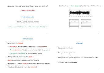
Overview Changes in mean Changes in spectrum Changes in dynamics and vibration-based SHM Conclusion Introduction Simulated data - One change ! 2 1 0 -1 -2 0 200 400 600 800 1000 1200 1400 1600 1800 2000 10 10 0 0 -10 -10 -20 -20 -30 -30 -40 -40 0 0.5 0 0.5

Overview Changes in mean Changes in spectrum Changes in dynamics and vibration-based SHM Conclusion Introduction Problems and issues Problems Detection of changes Stochastic models (static, dynamic) ← → uncertainties Parameterized models (physical interpretation, diagnostics) Damage ← → change in the parameter vector : θ 0 → θ 1 Many changes of interest are small Early detection of (small) deviations is useful Key issues Which function of the data should be handled ? 1 How to handle that function to make the decision ? 2

Overview Changes in mean Changes in spectrum Changes in dynamics and vibration-based SHM Conclusion Introduction Content Theory and algorithms Changes in the mean Changes in the spectrum Changes in the system dynamics and vibration-based SHM Application examples Handling the thermal effect in SHM 1 Aircraft flutter monitoring 2

Overview Changes in mean Changes in spectrum Changes in dynamics and vibration-based SHM Conclusion Key concepts - Independent data Likelihood ratio p θ ( y i ) Likelihood ln p θ 1 ( y i ) s i ∆ Log-likelihood ratio = p θ 0 ( y i ) E θ 0 ( s i ) 0 < E θ 1 ( s i ) 0 > � p θ 1 ( Y N i p θ 1 ( y i ) 1 ) ∆ Likelihood ratio Λ N = 1 ) = � p θ 0 ( Y N i p θ 0 ( y i ) ln Λ N = � N S N ∆ i = 1 s i Log-likelihood ratio =

Overview Changes in mean Changes in spectrum Changes in dynamics and vibration-based SHM Conclusion Key concepts - Independent data Hypothesis testing Hypotheses H 0 H 1 Simple Known parameter values θ 0 θ 1 Composite Unknown parameter values Θ 0 Θ 1 Simple hypotheses: Likelihood ratio test If Λ N ≥ λ or equivalently S N ≥ h : decide H 1 ; H 0 otherwise Composite hypotheses: Generalized likelihood ratio (GLR) test p � θ 1 ( Y N Λ N = sup θ 1 ∈ Θ 1 p θ 1 ( Y N 1 ) 1 ) � 1 ) = sup θ 0 ∈ Θ 0 p θ 0 ( Y N p � θ 0 ( Y N 1 ) Rule: Maximize the likelihoods w.r.t. unknown values of θ 0 and θ 1

Overview Changes in mean Changes in spectrum Changes in dynamics and vibration-based SHM Conclusion Key concepts - Independent data On-line change detection θ o θ 1 t o n 1 ? θ = θ 0 known ( 1 ≤ i ≤ k ) Hypothesis H 0  ( 1 ≤ i < t 0 ) θ 0  ∃ t 0 unknown s.t. Hypothesis H 1 θ =  ( t 0 ≤ i ≤ k ) θ 1 Alarm time t a : t a = min { k ≥ 1 : g k ≥ h } Wanted: decision function g k , onset time estimate ( � t 0 ) k

Overview Changes in mean Changes in spectrum Changes in dynamics and vibration-based SHM Conclusion Simple case: Known θ 1 CUSUM algorithm Ratio of likelihoods under H 0 and H 1 : � t 0 − 1 p θ 0 ( y i ) · � k � k i = t 0 p θ 1 ( y i ) i = t 0 p θ 1 ( y i ) i = 1 = Λ k = � k � k t 0 i = 1 p θ 0 ( y i ) i = t 0 p θ 0 ( y i ) Rule: Maximize the likelihood ratio w.r.t. the unknown onset time t 0 j − 1 k � � t 0 ) k ∆ p θ 0 ( y i ) · p θ 1 ( y i ) arg max ( � = 1 ≤ j ≤ k i = 1 i = j Λ k arg max = j 1 ≤ j ≤ k S k S k = ln Λ k ∆ arg max = j , j j 1 ≤ j ≤ k 1 ≤ j ≤ k S k = ln Λ k g k ∆ max = j t 0 ˆ

Overview Changes in mean Changes in spectrum Changes in dynamics and vibration-based SHM Conclusion Simple case: Known θ 1 CUSUM algorithm (Contd.) Lesson 1 1 ≤ j ≤ k S k g k ∆ max = j 1 ≤ j ≤ k S j 1 ≤ j ≤ k S j S k 1 = S k 1 − m k , m k ∆ 1 − min = min = 1 min { k ≥ 1 : S k t a 1 ≥ m k + h } Adaptative threshold = g k ( g k − 1 + s k ) + = � � + S k g k N k = N k − 1 · I ( g k − 1 ) + 1 ∆ = , k − N k + 1 t 0 ) k t a − N t a + 1 ( � Sliding window with adaptive size =

Overview Changes in mean Changes in spectrum Changes in dynamics and vibration-based SHM Conclusion Simple case: Known θ 1 CUSUM algorithm - Gaussian example � � − ( y i − µ ) 2 1 N ( µ, σ 2 ) , θ ∆ p θ ( y ) ∆ exp √ = µ, = 2 σ 2 2 π σ ln p µ 1 ( y i ) s i = p µ 0 ( y i ) � ( y i − µ 0 ) 2 − ( y i − µ 1 ) 2 � 1 = 2 σ 2 � � ν y i − µ 0 − ν ν ∆ = µ 1 − µ 0 change magnitude = , σ 2 2 k � S k y i : involves Integrator (with adaptive threshold) 1 i = 1

Overview Changes in mean Changes in spectrum Changes in dynamics and vibration-based SHM Conclusion Simple case: Known θ 1 CUSUM algorithm - Gaussian example (Contd.) 7 6 5 4 3 2 1 0 -1 -2 y k -3 0 5 10 15 20 25 30 35 40 45 50 10 0 -10 -20 -30 -40 S k -50 0 5 10 15 20 25 30 35 40 45 50 1 90 80 70 60 50 40 30 20 10 g k 0 0 5 10 15 20 25 30 35 40 45 50

Overview Changes in mean Changes in spectrum Changes in dynamics and vibration-based SHM Conclusion Composite case: Unknown θ 1 Unknown θ 1 - Algorithms Modified CUSUM algorithms Minimum magnitude of change Weighted CUSUM GLR algorithm Double maximization S k g k = max 1 ≤ j ≤ k sup j ( θ 1 ) θ 1 Gaussian case, additive faults: second maximization explicit

Overview Changes in mean Changes in spectrum Changes in dynamics and vibration-based SHM Conclusion Composite case: Unknown θ 1 Unknown θ 1 - Gaussian example Lesson 2 Introducing a minimum magnitude of change ν m Decreasing mean Increasing mean � � � � = � k = � k y i − µ 0 + ν m y i − µ 0 − ν m T k ∆ U k ∆ i = 1 i = 1 1 1 2 2 = max 1 ≤ j ≤ k T j = min 1 ≤ j ≤ k U j M k ∆ m k ∆ 1 1 t a = min { k ≥ 1 : M k − T k t a = min { k ≥ 1 : U k 1 ≥ h } 1 − m k ≥ h }

Overview Changes in mean Changes in spectrum Changes in dynamics and vibration-based SHM Conclusion Key concepts - Dependent data Conditional likelihood ratio p θ ( y i |Y i − 1 Cond. likelihood ) 1 ln p θ 1 ( y i |Y i − 1 ) s i ∆ 1 Log-likelihood ratio = p θ 0 ( y i |Y i − 1 ) 1 E θ 0 ( s i ) 0 < E θ 1 ( s i ) 0 > � i p θ 1 ( y i |Y i − 1 p θ 1 ( Y N ) 1 ) ∆ 1 Likelihood ratio Λ N = 1 ) = � p θ 0 ( Y N i p θ 0 ( y i |Y i − 1 ) 1 ln Λ N = � N S N ∆ i = 1 s i Log-likelihood ratio =

Overview Changes in mean Changes in spectrum Changes in dynamics and vibration-based SHM Conclusion Key concepts - Dependent data Which residuals ? Lesson 3 Residuals based on statistical inference Likelihood ratio : may be computationally complex Efficient score ∆ = likelihood sensitivity w.r.t. parameter Any other parameter estimating fonction Warning The innovation is OK for additive faults but NOT for multiplicative faults The innovation is NOT sufficient for monitoring the system dynamics

Overview Changes in mean Changes in spectrum Changes in dynamics and vibration-based SHM Conclusion Key concepts - Dependent data Building a residual Given θ 0 : reference parameter, known (or identified) Y k : N -size sample of new measurements Wanted A residual ζ significantly non zero when a change occurs Solution Residual ↔ Estimating function ζ N ( θ, Y N 1 ) Characterized by: E θ 0 ζ N ( θ, Y N 1 ) = 0 ⇐ ⇒ θ = θ 0

Overview Changes in mean Changes in spectrum Changes in dynamics and vibration-based SHM Conclusion Key concepts - Dependent data Designing the test Residual behavior Mean sensitivity J ( θ 0 ) and covariance Σ( θ 0 ) of ζ N ( θ 0 ) The residual is asymptotically Gaussian  N ( 0 , Σ( θ 0 )) if P θ 0   ζ N ( θ 0 ) →  Σ( θ 0 )) if P θ 0 + δθ N small change  N ( J ( θ 0 ) δθ, √ (On-board) χ 2 -test ζ T N Σ − 1 J ( J T Σ − 1 J ) − 1 J T Σ − 1 ζ N ≥ h Invariant / pre-multiplication of ζ with invertible gain. Noises and uncertainty on θ 0 taken into account

Overview Changes in mean Changes in spectrum Changes in dynamics and vibration-based SHM Conclusion Structural monitoring Vibration-based monitoring problem The excitation natural, not controlled not measured: buildings, bridges, offshore structures, rotating machinery, cars, trains, aircrafts nonstationary (e.g., turbulent) Questions How to detect and localize small damages ? Early ? On-board ?

Overview Changes in mean Changes in spectrum Changes in dynamics and vibration-based SHM Conclusion Structural monitoring Modelling  M ¨ Z ( s ) + C ˙ Z ( s ) + K Z ( s ) = ǫ ( s )  FE model:  Y ( s ) = L Z ( s ) ( M µ 2 + C µ + K ) Ψ µ = 0 , ψ µ = L Ψ µ  X k + 1 F X k + V k =  State space:  Y k H X k = F Φ λ = λ Φ λ , ϕ λ = H Φ λ ∆ e δµ = λ , ψ µ = ϕ λ � �� � � �� � modes mode shapes