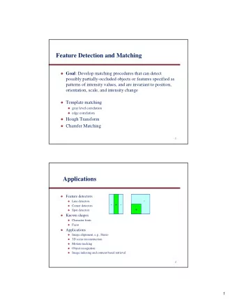
Feature Detection and Matching Applications Goal : Develop matching - PowerPoint PPT Presentation

Feature Detection and Matching Applications � Goal : Develop matching procedures that can detect � Feature detectors - � Line detectors possibly partially-occluded objects or features specified as - + - � Corner detectors patterns of intensity values, and are invariant to position, + � Spot detectors orientation, scale, and intensity change � Known shapes � Character fonts � Faces � Template matching � Applications � gray level correlation � Image alignment, e.g., Stereo � edge correlation � 3D scene reconstruction � Hough Transform � Motion tracking � Object recognition � Chamfer Matching � Image indexing and content-based retrieval 1 2 Example: Build a Panorama How do we build panorama? � We need to match (align) images M. Brown and D. G. Lowe. Recognising Panoramas. ICCV 2003 3 4 1

Matching with Features Matching with Features • Detect feature points in both images • Detect feature points in both images • Find corresponding pairs 5 6 Matching with Features Matching with Features • Detect feature points in both images � Problem 1: • Find corresponding pairs � Detect the same point independently in both images • Use these pairs to align images no chance to match! We need a repeatable detector 7 8 2

Harris Corner Detector Matching with Features � Problem 2: � For each point correctly recognize the corresponding one ? We need a reliable and distinctive descriptor 9 10 C. Harris, M. Stephens, “A Combined Corner and Edge Detector,” 1988 Harris Detector: Basic Idea The Basic Idea � We should easily recognize the point by looking through a small window � Shifting a window in any direction should give a large change in response “flat” region: “edge”: “corner”: no change in no change along significant change all directions the edge direction in all directions 11 12 3

Harris Detector: Mathematics Harris Detector: Mathematics Expanding E ( u , v ) in a 2 nd order Taylor series, we have, for small Change of intensity for the shift [ u,v ]: shifts, [ u,v ], a bilinear approximation: ∑ [ ] 2 = + + − E u v ( , ) w x y ( , ) I x ( u y , v ) I x y ( , ) ⎡ ⎤ u [ ] ≅ E u v ( , ) u v , M ⎢ ⎥ x y , ⎣ ⎦ v Window Shifted Intensity function intensity where M is a 2 × 2 matrix computed from image derivatives: ⎡ ⎤ 2 I I I ∑ = x x y ⎢ ⎥ M w x y ( , ) Window function w ( x,y ) = or 2 ⎢ I I I ⎥ ⎣ ⎦ x y , x y y 1 in window, 0 outside Gaussian 16 17 Selecting Good Features Harris Detector: Mathematics Intensity change in shifting window: eigenvalue analysis ⎡ ⎤ u [ ] λ 1 , λ 2 – eigenvalues of M ≅ E u v ( , ) u v , M ⎢ ⎥ ⎣ ⎦ v direction of the fastest change Ellipse E(u,v) = const direction of the slowest change ( λ max ) -1/2 ( λ min ) -1/2 λ 1 and λ 2 are large 18 19 4

Selecting Good Features Selecting Good Features large λ 1 , small λ 2 small λ 1 , small λ 2 20 21 Harris Detector: Mathematics Harris Detector: Mathematics λ 2 Measure of corner response: “Edge” λ 2 >> λ 1 “Corner” ( ) 2 = − Classification of R det M k trace M λ 1 and λ 2 both large, image points using λ 1 ~ λ 2 ; eigenvalues of M : E increases in all directions = λ λ det M 1 2 = λ + λ trace M 1 2 λ 1 and λ 2 are small; “Edge” E is almost constant “Flat” λ 1 >> λ 2 in all directions region k is an empirically-determined constant; e.g., k = 0.05 λ 1 22 23 5

Harris Detector: Mathematics Harris Detector λ 2 “Edge” “Corner” � The Algorithm: • R depends only on R < 0 � Find points with large corner response function R eigenvalues of M ( R > threshold) • R is large for a corner R > 0 � Take the points of local maxima of R (for localization) • R is negative with large magnitude for an edge • | R | is small for a flat region “Flat” “Edge” |R| small R < 0 λ 1 24 25 Harris Detector: Example Harris Detector: Example Compute corner response R 26 27 6

Harris Detector: Example Harris Detector: Example Find points with large corner response: R > threshold Take only the points of local maxima of R 28 29 Harris Detector: Example Harris Detector: Example Interest points extracted with Harris (~ 500 points) 30 31 7

Harris Detector: Summary Harris Detector: Some Properties � Rotation invariance � Average intensity change in direction [ u,v ] can be expressed as a bilinear form: ⎡ ⎤ u [ ] ≅ E u v ( , ) u v , M ⎢ ⎥ ⎣ ⎦ v � Describe a point in terms of eigenvalues of M : measure of corner response: Ellipse rotates but its shape (i.e., eigenvalues) ( ) 2 = λ λ − λ + λ R k remains the same 1 2 1 2 � A good (corner) point should have a large intensity change Corner response R is invariant to image rotation in all directions , i.e., R should be a large positive value 32 33 Harris Detector Properties: Rotation Invariance Harris Detector Properties: Rotation Invariance [Comparing and Evaluating Interest Points, Schmid, Mohr & Bauckhage, ICCV 98] 34 35 C.Schmid et.al. “Evaluation of Interest Point Detectors”. IJCV 2000 8

Harris Detector Properties: Perspective Changes Harris Detector Properties: Intensity Changes � Partial invariance to affine intensity change � Only derivatives are used ⇒ invariance to intensity shift I → I + b � Intensity scale: I → a I R R threshold [Comparing and Evaluating Interest Points, Schmid, Mohr & Bauckhage, ICCV 98] x (image coordinate) x (image coordinate) 36 37 Harris Detector Properties: Scale Changes Harris Detector: Some Properties � But not invariant to image scale � Quality of Harris detector for different scale changes Repeatability rate: # correspondences # possible correspondences Fine scale: All points will Coarse scale: Corner be classified as edges 38 39 C. Schmid et al., “Evaluation of Interest Point Detectors,” IJCV 2000 9

Tomasi and Kanade’s Corner Detector Corner Detection (cont.) � Diagonalize M converting it to the form ⎡ λ ⎤ � Idea: Intensity surface has 2 directions with significant 0 = 1 ⎢ ⎥ M intensity discontinuities λ ⎣ 0 ⎦ � Image gradient [ I x , I y ] T gives information about direction 2 and magnitude of one direction, but not two � Eigenvalues λ 1 and λ 2 , λ 1 ≥ λ 2 , give measure of the edge strength (i.e., magnitude) of the two strongest, perpendicular edge directions (specified � Compute 2 x 2 matrix by the eigenvectors of M ) ∑ ∑ ⎡ ⎤ 2 � If λ 1 ≈ λ 2 ≈ 0, then p ’s neighborhood is approximately constant intensity I I I x x y ⎢ ⎥ = Q Q � If λ 1 > 0 and λ 2 ≈ 0, then single step edge in neighborhood of p M ⎢ ∑ ∑ ⎥ 2 I I I � If λ 2 > threshold and no other point within p ’s neighborhood has greater ⎢ ⎥ x y y ⎣ ⎦ Q Q value of λ 2 , then mark p as a corner point where Q is a 2 n +1 x 2 n +1 neighborhood of a given point p 40 41 Tomasi and Kanade Corner Algorithm Results � Compute the image gradient over entire image � For each image point p : � form the matrix M over (2N+1) x (2N+1) neighborhood Q of p � compute the smallest eigenvalue of M � if eigenvalue is above some threshold, save the coordinates of p in a list L � Sort L in decreasing order of eigenvalues � Scanning the sorted list top to bottom: For each current point, p , delete all other points on the list that belong to the neighborhood of p 42 43 10

Results Results 44 45 Moravec’s Interest Operator � Compute four directional variances in horizontal, vertical, 3 2 ∑∑ = + + − + + + 2 ( ( , ) ( 1 , )) V P x i y j P x i y j diagonal and anti-diagonal directions for each 4 x 4 h = = j 0 i 0 window 2 3 ∑∑ � If the minimum of four directional variances is a local = + + − + + + 2 V ( P ( x i , y j ) P ( x i , y j 1 )) maximum in a 12 x 12 overlapping neighborhood, then v = = 0 0 j i that window (point) is “interesting” 2 2 ∑∑ = + + − + + + + 2 ( ( , ) ( 1 , 1 )) V P x i y j P x i y j d = = j 0 i 0 2 3 ∑∑ = + + − + − + + 2 V ( P ( x i , y j ) P ( x i 1 , y j 1 )) a = = 0 1 j i 46 47 11

= V ( x , y ) min( V ( x , y ), V ( x , y ), V ( x , y ), V ( x , y )) h v d a ⎧ 1 , if ( , ) is a local max V x y = ⎨ ( , ) I x y ⎩ 0 , otherwise 48 49 Models of Image Change Invariant Local Features � Goal: Detect the same interest points regardless of � Geometry image changes due to translation, rotation, scale, etc. � Rotation � Similarity (rotation + uniform scale) � Affine (scale dependent on direction) valid for: orthographic camera, locally planar object � Photometry � Affine intensity change ( I → a I + b ) 50 51 12