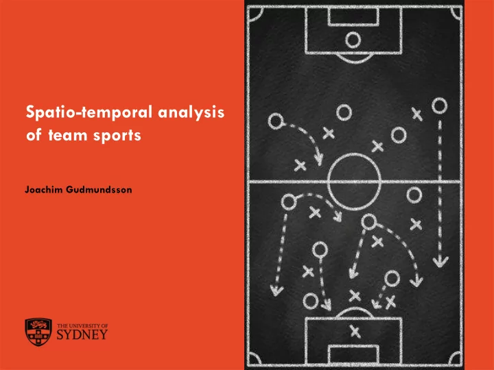
of team sports Joachim Gudmundsson The University of Sydney Page 1 - PowerPoint PPT Presentation

Spatio-temporal analysis of team sports Joachim Gudmundsson The University of Sydney Page 1

Team sport analysis Talk is partly based on: Joachim Gudmundsson and Michael Horton Spatio-Temporal Analysis of Team Sports ACM Computing Surveys, 50(2), 2017 Invasion sports: Two teams trying to score against each other. For example, football, American football, Australian football, ice hockey, handball, basketball,… Spatio-temporal data as primary input. This talk will focus on algorithmic issues. The University of Sydney Page 2

Overview of major approaches The University of Sydney Page 3

Input data TEAM Player X Player Y PLAYER NAME NAME MATCH FIXTURE HALF TIME Position Position Bacary Sagna Arsenal Arsenal v Bolton First half 0 -1745 1897 Bacary Sagna Arsenal Arsenal v Bolton First half 0.1 -1748 1902 Bacary Sagna Arsenal Arsenal v Bolton First half 0.2 -1751 1907 Bacary Sagna Arsenal Arsenal v Bolton First half 0.3 -1754 1913 Bacary Sagna Arsenal Arsenal v Bolton First half 0.4 -1757 1918 Bacary Sagna Arsenal Arsenal v Bolton First half 0.5 -1760 1923 Bacary Sagna Arsenal Arsenal v Bolton First half 0.6 -1763 1929 83.8 Touch DIABY Abou 24 -13 84.8 Block BASHAM Chris 25 -12 86.7 Pass MCCANN Gavin 23 -4 88 Foul GARDNER Ricardo DENILSON 15 -8 109 Direct Free Kick Pass JAASKELAINEN Jussi 14 -7 111.2 Header CLICHY Gael -26 -11 113 Touch CLICHY Gael -26 -17 The University of Sydney Page 4

Input data The University of Sydney Page 5

History: Sports analysis – Box scores for baseball started in the 1850s. – Manual notation of football games started in the 1950s. – Moneyball-era in baseball – Similar development in basketball in the last 10 years – Human observations are unreliable. Franks and Miller [1986] showed that expert observers’ recollection of significant match events is as low as 42%. – Automated tracking of sport players started in the early 2000s. – Nowadays a number of automatic tracking systems for football, ice hockey and basketball (not much in rugby, AFL and handball). The University of Sydney Page 6

Outline – Playing area subdivision – Dominant regions – Applications – Modelling player interaction as social networks – Data mining – Labelling – Identifying formations and plays – Trajectory analysis – Sport-specific trajectory problems The University of Sydney Page 7

Playing area subdivision: Intensity maps First attempts to analyze trajectory data… The University of Sydney Page 8

Playing area subdivision: Intensity maps And more… The University of Sydney Page 9

Playing area subdivision: Dominant region A team’s ability to control space is considered a key factor in the team’s performance. Dominant region [Taki and Hasegawa’99] The dominant region of a player p is the region of the pitch that player p can reach before any other player. Reach? p The University of Sydney Page 10

Playing area subdivision: Dominant region Dominant region [Taki and Hasegawa’99] The dominant region of a player p is the region of the pitch that player p can reach before any other player. DR(p)={x | d(x,p ) ≤ d( x,q) for all q  p} If d(  ,  ) = Euclidean distance then Dominant region = Voronoi diagram [Descartes 1644] The University of Sydney Page 11

Playing area subdivision: Movement model [Taki and Hasegawa’99] Linear interpolation of acceleration in all directions. [Fujimura and Sugihara’05] Introduced a resistive force to decrease acceleration. The University of Sydney Page 12

Playing area subdivision: Movement models Simple way to model? The University of Sydney Page 13

Playing area subdivision: Movement model Movement model Circle model Ellipse model The University of Sydney Page 14

Playing area subdivision: Movement model Movement model A bisector in the ellipse model The University of Sydney Page 15

Playing area subdivision: Movement model Dominant region The University of Sydney Page 16

Playing area subdivision: Movement model Movement model Model: Turning cost + Euclidean distance The University of Sydney Page 17

Playing area subdivision: Movement model Movement model [Taki & Hasegawa’00] The University of Sydney Page 18 1

Playing area subdivision: Movement model Movement model [De Berg, Haverkort and Horton’17] The University of Sydney Page 19

Playing area subdivision: Movement model Open problem 1: Define a motion function that faithfully models player movement and is tractable for computation. The University of Sydney Page 20

Playing area subdivision: Passing evaluation A player p is open for a pass if there is some direction and (reasonable) speed that the ball can be passed, such that p can intercept the ball before any other player. The University of Sydney Page 21

Playing area subdivision: Passing evaluation Passability with a fixed pass speed (20m/s). The University of Sydney Page 22

Playing area subdivision: Passing evaluation The existing models for determining whether a player is open to receive a pass only consider passes made along the shortest path between passer and receiver and where the ball is moving at constant velocity. Open problem 2: Develop a more realistic model that allows for aerial passes, effects of ball-spin, and variable velocities. The University of Sydney Page 23

Playing area subdivision: Spatial pressure Spatial pressure of player [Taki et al. ‘96] Spatial pressure for a player p is related to the fraction P of the disk of radius r centred at p that lies within dominant region of opposing players, i.e. m(1-P)+(1-m)(1-d/D), where d – distance between p and the ball D – distance from p to point furthest from p on pitch m – preset weight The University of Sydney Page 24

Playing area subdivision: Spatial pressure Spatial pressure of player The University of Sydney Page 25

Playing area subdivision: Spatial pressure Spatial pressure of player The University of Sydney Page 26

Playing area subdivision: Spatial pressure Spatial pressure of player The University of Sydney Page 27

Playing area subdivision: Spatial pressure Spatial pressure of player The University of Sydney Page 28

Playing area subdivision: Spatial pressure Spatial pressure of player The University of Sydney Page 29

Playing area subdivision: Spatial pressure The definition of spatial pressure is very simple. Open problem 3: Can a model that incorporates the direction the player is facing or the direction of pressuring opponents be devised and experimentally tested? The University of Sydney Page 30

Modelling team sports as social networks Understanding the interaction between players is one of the most important and complex problems in sports science. Numerous papers apply social network analysis to team sports. Passing network Transition network The University of Sydney Page 31

Modelling team sports as social networks Many properties of passing networks have been studied: – Centrality – Degree – Betweenness – Closeness – Eigenvector centrality and Pagerank – Clustering coefficients – Density and heterogeneity – Entropy, topological depth, Price-of-Anarchy The University of Sydney Page 32

Modelling team sports as social networks [Grund’12] Studied degree centrality on networks generated from 283k passes. Conclusion: High level of centralization decreases team performance. Open problem 4: A systematic study reviewing various centrality and clustering measures against predefined criteria, and on a large dataset would be a useful contribution to the field. The University of Sydney Page 33

Modelling team sports as social networks [Balkundi and Harrison’06] Density-performance hypothesis. More passes will make a team stronger. Open problem 5: The density-performance hypothesis suggests an interesting metric of team performance. Can this hypothesis be tested scientifically? The University of Sydney Page 34

Data mining: Labelling events – Evaluate passes (good/bad) [Horton et al.’15] – Identify teams (based on formation) [Bialkowski et al.’14] – Predict rebounds (offensive/defensive team) [Maheswaran et al’12] The University of Sydney Page 35

Data mining: Labelling passes Examples of features: Area of receiving player’s dominant region • • The net change in the area of receiving player’s dominant region • Total area of the team’s dominant region The net change of the total area of the team’s dominant region • Passer Pressure • Receiver Pressure • • Passer-Receiver Pressure Net Change The University of Sydney Page 36

Data mining: Labelling passes Extracted feature vectors from 2932 passes from four matches • Pass examples were labelled by humans watching video of match • Class imbalance: • Class Rel. frequency Count Good 0.066 193 OK 0.789 2314 Bad 0.145 425 SVN classifier: Accuracy 90.8% which is similar to a human observer • Features based on dominating region are among the most • important [Horton et al.’15] The University of Sydney Page 37