Normalized Cut Method for Image Segmentation J. Shi and J. Malik, - PDF document

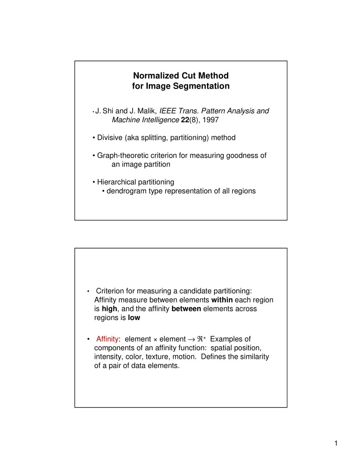
Normalized Cut Method for Image Segmentation • J. Shi and J. Malik, IEEE Trans. Pattern Analysis and Machine Intelligence 22 (8), 1997 • Divisive (aka splitting, partitioning) method • Graph-theoretic criterion for measuring goodness of an image partition • Hierarchical partitioning • dendrogram type representation of all regions Criterion for measuring a candidate partitioning: • Affinity measure between elements within each region is high , and the affinity between elements across regions is low Affinity: element × element → ℜ + Examples of • components of an affinity function: spatial position, intensity, color, texture, motion. Defines the similarity of a pair of data elements. 1

Affinity (Similarity) Measures • Intensity 2 2 2 ( ) ( ) / − x − y σ aff ( x , y ) I I = e I • Distance 2 2 2 x y / − − σ aff( x , y ) = e d • Color • Texture • Motion Problem Formulation • Given an undirected graph G = ( V , E ), where V is a set of nodes, one for each data element (e.g., pixel), and E is a set of edges with weights representing the affinity between connected nodes • Find the image partition that maximizes the “association” within each region and minimizes the “disassociation” between regions • Finding the optimal partition is NP-complete 2

• Let A, B partition G. Therefore, A ∪ B = V, and A ∩ B = ∅ • The affinity or similarity between A and B is defined as � w cut (A,B) = ij ∈ , ∈ i A j B = total weight of edges removed • The optimal bi-partition of G is the one that minimizes cut • Cut is biased towards small regions • So, instead define the normalized similarity, called the normalized-cut (A,B), as ( , ) ( , ) cut A B cut B A ( , ) = + ncut A B ( , ) ( , ) assoc A V assoc B V � w where assoc (A,V) = ik ∈ , ∈ i A k V = total connection weight from nodes in A to all nodes in G • Ncut measures the disimilarity between regions (“ disassociation ” measure) • Ncut removes the bias based on region size (usually) 3

• Similarly, define the “ normalized association :” ( , ) ( , ) assoc A A assoc B B ( , ) = + nassoc A B ( , ) ( , ) assoc A V assoc B V • Nassoc measures how similar, on average, nodes within the groups are to each other • New goal: Find the bi-partition that minimizes ncut (A,B) and maximizes nassoc (A,B) • But, it can be proved that ncut (A,B) = 2 – nassoc (A,B), so we can just minimize ncut : y = arg min ncut 1 , if node ∈ i A • Let y be a P = |V| dimensional vector where { − = y i 1 , otherwise � d ) ( = i w • Let ij j define the affinity of node i with all other nodes • Let D = P x P diagonal matrix: 0 ... 0 � d � 1 � � 0 ... 0 d � � 2 D = “degree matrix” � ... � � � 0 0 ... d � � P 4

• Let A = P x P symmetric matrix: ... � w w w � 11 12 1 P � � ... w w w � � 21 22 2 P A = “affinity matrix” � ... � � � ... w w w � � • It can be shown that P 1 P 2 PP y = arg min x ncut ( x ) T ( ) y D − A y arg min subject to y T D1 0 = = y y T Dy • Relaxing the constraint on y so as to allow it to have real values means that we can approximate the solution by solving an equation of the form: ( D – A ) y = λ Dy • The solution, y , is an eigenvector of ( D – A ) • An eigenvector is a characteristic vector of a matrix and specifies a segmentation based on the values of its components; similar points will hopefully have similar eigenvector components. • Theorem: If M is any real, symmetric matrix and x is orthogonal to the j -1 smallest eigenvectors x 1 , …, x j -1 , then x T Mx / x T x is minimized by the next smallest eigenvector x j and its minimum value is the eigenvalue λ j 5

• Smallest eigenvector is always 0 because A = V , B ={} means ncut ( A , B )=0 • Second smallest eigenvector is the real-valued y that minimizes ncut • Third smallest eigenvector is the real-valued y that optimally sub-partitions the first two regions • Etc. • Note: Converting from the real-valued y to a binary- valued y introduces errors that will propagate to each sub-partition NCUT Segmentation Algorithm 1. Set up problem as G = ( V , E ) and define affinity matrix A and degree matrix D 2. Solve ( D – A ) x = λ Dx for the eigenvectors with the smallest eigenvalues 3. Let x 2 = eigenvector with the 2 nd smallest eigenvalue λ 2 4. Threshold x 2 to obtain the binary-valued vector x´ 2 such that ncut ( x´ 2 ) ≥ ncut ( x t 2 ) for all possible thresholds t 5. For each of the two new regions, if ncut < threshold T, then recurse on the region 6

Comments on the Algorithm • Recursively bi-partitions the graph instead of using the 3 rd , 4 th , etc. eigenvectors for robustness reasons (due to errors caused by the binarization of the real-valued eigenvectors) • Solving standard eigenvalue problems takes O (P 3 ) time • Can speed up algorithm by exploiting the “locality” of affinity measures, which implies that A is sparse (non- zero values only near the diagonal) and ( D – A ) is sparse. This leads to a O (P √ P) time algorithm Example: 2D Point Set 7

Eigenvalues and Eigenvectors 8

Example 2: A Grayscale Image 9

Eigenvalues and Eigenvectors Discretizing an Eigenvector 10

Partitioning stops when histogram is not bimodal 11

Some Example Results 12