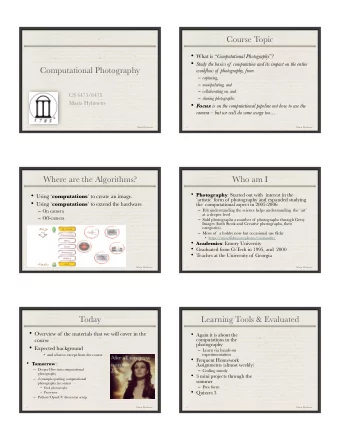
Computational Photography Si Lu Spring 2018 - PowerPoint PPT Presentation

Computational Photography Si Lu Spring 2018 http://web.cecs.pdx.edu/~lusi/CS510/CS510_Computati onal_Photography.htm 05/10/2018

Last Time o Image segmentation n Normalized cut and segmentation 2

Today o Segmentation n Interactive image segmentation Magic Wand GrabCut Intelligent Scissors (Photoshop) Rother et al. 2004 Mortensen and Barrett (1995) User Input Result Images from Rother et al. 2004 3

Start o Segmentation n Interactive image segmentation Images from Sun et al. 2004 4

Segmentation by Graph Cut o Interactive image segmentation using graph cut o Binary label: foreground vs. background o User labels some pixels n usually sparser F F B o Exploit F F B n Statistics of known Fg & Bg F B B n Smoothness of label o Turn into discrete graph optimization n Graph cut (min cut / max flow) Slide credit: Y.Y. Chuang 5

Energy function o Segmentation as Labeling one value per pixel, F or B n o Energy(labeling) = data + smoothness One labeling n Very general situation (ok, not best) n Will be minimized o Data: for each pixel n Probability that this color belongs to F (resp. B) o Smoothness (aka regularization): Data per neighboring pixel pair Penalty for having different label n n Penalty is down-weighted if the two pixel colors are very different n Similar in spirit to bilateral filter Smoothness Slide credit: F. Durand 6

Data term o A.k.a regional term (because integrated over full region) o D(L)=  i -log h[L i ](C i ) o Where i is a pixel L i is the label at i (F or B), C i is the pixel value h[L i ] is the histogram of the observed Fg (resp Bg) o Note the minus sign Slide credit: F. Durand 7

Hard constraints o The user has provided some labels o The quick and dirty way to include constraints into optimization is to replace the data term by a huge penalty if not respected. o D(L_i)=0 if respected o D(L_i)=K if not respected n e.g. K= #pixels Slide credit: F. Durand 8

Smoothness term o a.k.a boundary term, a.k.a. regularization o S(L)=  {j, i} in N B(C i ,C j )  (L i -L j ) o Where i,j are neighbors n e.g. 8-neighborhood (but I show 4 for simplicity) o  (L i -L j ) is 0 if L i =L j , 1 otherwise o B(C i ,C j ) is high when C i and C j are similar, low if there is a discontinuity between those two pixels e.g. exp(-||C i -C j || 2 /2  2 ) n where  can be a constant n or the local variance o Note positive sign Slide credit: F. Durand 9

Optimization o E(L)=D(L)+  S(L) o  is a black-magic constant o Find the labeling that minimizes E o In this case, how many possibilities? n 2 9 (512) n We can try them all! n What about megapixel images? Slide credit: F. Durand 10

Labeling as a graph problem o Each pixel = node o Add two nodes F & B o Labeling: link each pixel to either F or B F Desired result B Slide credit: F. Durand 11

Data term o Put one edge between each pixel and F & B o Weight of edge = minus data term n Don ’ t forget huge weight for hard constraints F n Careful with sign B Slide credit: F. Durand 12

Smoothness term o Add an edge between each neighbor pair o Weight = smoothness term F B Slide credit: F. Durand 13

Min cut o Energy optimization equivalent to min cut o Cut: remove edges to disconnect F from B o Minimum: minimize sum of cut edge weight F cut B Slide credit: F. Durand 14

Min cut <=> labeling o In order to be a cut: n For each pixel, either the F or G edge has to be cut o In order to be minimal F n Only one edge label cut per pixel can be cut (otherwise could be added) B Slide credit: F. Durand 15

Computing a multiway cut o With 2 labels: classical min-cut problem n Solvable by standard flow algorithms o polynomial time in theory, nearly linear in practice o Code: C++ from OpenCV n Matlab wrapper: http://www.wisdom.weizmann.ac.il/~bagon/matlab.html n More than 2 terminals: NP-hard [Dahlhaus et al. , STOC ‘ 92] Code: http://vision.ucla.edu/~brian/gcmex.html o Efficient approximation algorithms exist n Within a factor of 2 of optimal n Computes local minimum in a strong sense o even very large moves will not improve the energy Yuri Boykov, Olga Veksler and Ramin Zabih, Fast Approximate Energy n Minimization via Graph Cuts, International Conference on Computer Vision, September 1999. Slide credit: Y.Y. Chuang 16

GrabCut – Interactive Foreground Extraction 1

Input : Image Output : Segmentation Parameters: Colour ,Coherence Energy: Optimization: GrabCut – Interactive Foreground Extraction 4

Cut: separating source and sink; Energy: collection of edges Min Cut: Global minimal enegry in polynomial time GrabCut – Interactive Foreground Extraction 5

? User Initialisation Graph cuts to K-means for learning infer the colour distributions segmentation GrabCut – Interactive Foreground Extraction 6

Guaranteed to converge 1 2 3 4 Result Energy after each Iteration GrabCut – Interactive Foreground Extraction 7

R R Iterated Foregroun Foregroun d & graph cut d Backgroun d G Backgroun Backgroun G d d Gaussian Mixture Model (typically 5-8 components) GrabCut – Interactive Foreground Extraction 8

An object is a coherent set of pixels: Blake et al. (2004): Learn jointly GrabCut – Interactive Foreground Extraction 9

… GrabCut completes automatically GrabCut – Interactive Foreground Extraction 10

Camouflage & Fine structure No telepathy Low Contrast Initial Rectangle Initial Result GrabCut – Interactive Foreground Extraction 11

Available online: http://research.microsoft.com/vision/cambridge/segmentation/ GrabCut – Interactive Foreground Extraction 12

Boykov and Jolly (2001) GrabCut User Input Result Error Rate: 1.87% Error Rate: 1.81% Error Rate: 1.32% Error Rate: 1.25% Error Rate: 0.72% Error Rate: 0.72% GrabCut – Interactive Foreground Extraction 13

Intelligent Scissors Graph Cuts LazySnapping Magic Wand GrabCut Mortensen and Boykov and Li et al. (2004) (198?) Rother et al. Barrett (1995) Jolly (2001) (2004) GrabCut – Interactive Foreground Extraction 22

Interactive Digital Photomontage o Combining multiple photos o Find seams using graph cuts o Combine gradients and integrate Aseem Agarwala, Mira Dontcheva, Maneesh Agrawala, Steven Drucker, Alex Colburn, Brian Curless, David Salesin, Michael Cohen, “Interactive Digital Photomontage”, SIGGRAPH 2004 Slide credit: Y.Y. Chuang 30

Slide credit: Y.Y. Chuang 31

Slide credit: Y.Y. Chuang 32

Slide credit: Y.Y. Chuang 33

Slide credit: Y.Y. Chuang 34

Slide credit: Y.Y. Chuang 35

Slide credit: Y.Y. Chuang 36

photomontage set of originals Slide credit: Y.Y. Chuang 37

Source images Brush strokes Computed labeling Composite Slide credit: Y.Y. Chuang 38

Brush strokes Computed labeling Slide credit: Y.Y. Chuang 39

Next Time o Matting 40