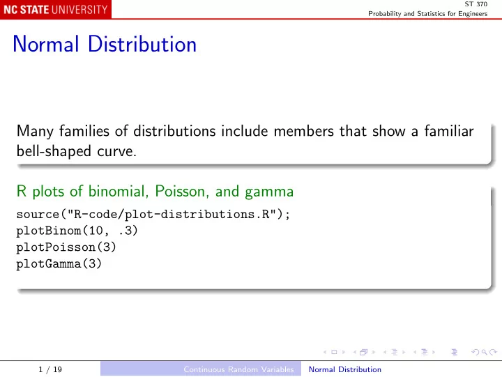
Normal Distribution Many families of distributions include members - PowerPoint PPT Presentation

ST 370 Probability and Statistics for Engineers Normal Distribution Many families of distributions include members that show a familiar bell-shaped curve. R plots of binomial, Poisson, and gamma source("R-code/plot-distributions.R"); plotBinom(10, .3) plotPoisson(3) plotGamma(3) 1 / 19 Continuous Random Variables Normal Distribution

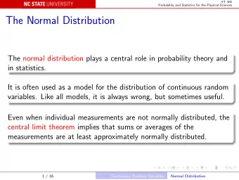
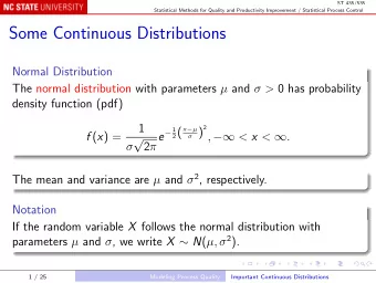
ST 370 Probability and Statistics for Engineers In each case, the underlying curve is a normal or Gaussian density function. If X has a Gaussian distribution, and E ( X ) = µ, V ( X ) = σ 2 , then the probability density function of X is 1 − ( x − µ )2 f X ( x ) = √ e . 2 σ 2 σ 2 π We write X ∼ N ( µ, σ 2 ): plotGaussian(mu = 2, sigma = 0.5) 2 / 19 Continuous Random Variables Normal Distribution

ST 370 Probability and Statistics for Engineers The standard normal distribution has µ = 0 and σ = 1; the probability density function simplifies to 1 − x 2 ϕ ( x ) = √ e 2 2 π If X ∼ N ( µ, σ 2 ) and Z = X − µ , σ then Z follows the standard normal distribution: Z ∼ N (0 , 1). Conversely, if Z ∼ N (0 , 1) and X = µ + σ Z , then X ∼ N ( µ, σ 2 ). 3 / 19 Continuous Random Variables Normal Distribution

ST 370 Probability and Statistics for Engineers Cumulative distribution function The cumulative distribution function of N (0 , 1) is written � x Φ( x ) = ϕ ( u ) du . −∞ It cannot be written in closed form, but is tabulated and programmed in most languages, such as the pnorm() function in R: curve(pnorm(x), from = -3, to = 3) 4 / 19 Continuous Random Variables Normal Distribution

ST 370 Probability and Statistics for Engineers Example: Normally distributed current The measured current X in a wire is normally distributed with mean µ = 10 mA and standard deviation σ = 2 mA. What is the probability that X > 13 mA? P ( X > 13) = 1 − P ( X ≤ 13) � X − 10 ≤ 13 − 10 � = 1 − P 2 2 = 1 − P ( Z ≤ 1 . 5) = 1 − Φ(1 . 5) . 1 - pnorm(1.5) # or more simply pnorm(13, mean = 10, sd = 2, lower.tail = FALSE) 5 / 19 Continuous Random Variables Normal Distribution

ST 370 Probability and Statistics for Engineers What is the probability that the current is between 9 and 11 mA? P (9 < X ≤ 11) = P ( X ≤ 11) − P ( X ≤ 9) � 11 − 10 � � 9 − 10 � = Φ − Φ 2 2 = Φ(0 . 5) − Φ( − 0 . 5) = Φ(0 . 5) − [1 − Φ(0 . 5)] = 2Φ(0 . 5) − 1 2 * pnorm(0.5) - 1 # or, since pnorm covers negative numbers, pnorm(0.5) - pnorm(-0.5) # or even pnorm(11, mean = 10, sd = 2) - pnorm(9, mean = 10, sd = 2) 6 / 19 Continuous Random Variables Normal Distribution

ST 370 Probability and Statistics for Engineers Normal Approximations Many families of distributions include members that show a familiar bell-shaped curve. The Gaussian distribution can be used to make approximate probability statements for the corresponding members of those families. In each case, we begin by standardizing the variable. 7 / 19 Continuous Random Variables Normal Approximations

ST 370 Probability and Statistics for Engineers Example: Binomial distribution Suppose that X has the binomial distribution with parameters n and p : X ∼ Bin( n , p ). Then E ( X ) = np , and V ( X ) = np (1 − p ) , so X − np Z = � np (1 − p ) is the corresponding standardized variable, with expected value 0 and standard deviation 1. 8 / 19 Continuous Random Variables Normal Approximations

ST 370 Probability and Statistics for Engineers Then if n is large and p is not close to either 0 or 1, the distribution of Z is close to the standard normal distribution. To be precise, P ( Z ≤ z ) ≈ Φ( z ) , and hence � � x − np P ( X ≤ x ) = P Z ≤ � np (1 − p ) � � x − np ≈ Φ . � np (1 − p ) 9 / 19 Continuous Random Variables Normal Approximations

ST 370 Probability and Statistics for Engineers Continuity correction The approximation is usually used with x an integer, and in that case P ( X ≤ x ) = P ( X ≤ x + 0 . 5) and � � x + 0 . 5 − np P ( X ≤ x ) ≈ Φ � np (1 − p ) is found to give a closer approximation to the exact probability. 10 / 19 Continuous Random Variables Normal Approximations

ST 370 Probability and Statistics for Engineers Of course, P ( X > x ) = 1 − P ( X ≤ x ) is approximated by � � x + 0 . 5 − np P ( X > x ) ≈ 1 − Φ . � np (1 − p ) 11 / 19 Continuous Random Variables Normal Approximations

ST 370 Probability and Statistics for Engineers But P ( X ≥ x ) = P ( X > x − 1) is approximated by � � x − 1 + 0 . 5 − np P ( X ≥ x ) ≈ 1 − Φ � np (1 − p ) � � x − 0 . 5 − np = 1 − Φ . � np (1 − p ) When the inequality is inclusive ( ≤ or ≥ ), the sign of the correction term ± 0 . 5 is chosen to increase the approximating probability. 12 / 19 Continuous Random Variables Normal Approximations

ST 370 Probability and Statistics for Engineers Example: Poisson distribution Suppose that X has the Poisson distribution with parameter θ : X ∼ Poisson( θ ). Then E ( X ) = V ( X ) = θ, so Z = X − θ √ θ is the corresponding standardized variable, with expected value 0 and standard deviation 1. 13 / 19 Continuous Random Variables Normal Approximations

ST 370 Probability and Statistics for Engineers Then if θ is large, the distribution of Z is close to the standard normal distribution. The approximation is used in the same way as for the binomial distribution, including the use of a continuity correction: � x + 0 . 5 − θ � P ( X ≤ x ) ≈ Φ √ , θ and so on. 14 / 19 Continuous Random Variables Normal Approximations

ST 370 Probability and Statistics for Engineers How large is large enough? You will sometimes read that these approximations are good if: np > 5 and n (1 − p ) > 5, in the binomial case; θ > 5 in the Poisson case. However, the approximation error can be as great as 0.03, so you are guaranteed no more than a rough approximation. Modern software makes it easy to use “exact” calculations (or at least much more accurate approximations), so these approximations are more useful in understanding the reason for the ubiquitous bell curve than in actual computation. 15 / 19 Continuous Random Variables Normal Approximations

ST 370 Probability and Statistics for Engineers The Gaussian distribution in the real world The central limit theorem (CLT) explains why the Gaussian distribution appears in theory. It states essentially that any random variable that is the sum of many small, independent contributions is approximately Gaussian. For instance, a binomial random variable is the sum of the success indicators for each trial. In many real world measurement systems, the random measurement noise does consist of the sum of many small perturbations, and by the CLT could be expected to be approximately Gaussian. But it is only an approximation, and often not a good one! 16 / 19 Continuous Random Variables Normal Approximations

ST 370 Probability and Statistics for Engineers Lognormal Distribution The Gaussian distribution is often used as a model for a measured physical quantity. But every Gaussian distribution has a positive probability of negative values, which is a deficiency if the physical quantity is always positive. One alternative that is often used is the lognormal distribution. 17 / 19 Continuous Random Variables Lognormal Distribution

ST 370 Probability and Statistics for Engineers Suppose that W ∼ N ( θ, ω 2 ), and that X = exp( W ); then conversely W = log( X ), and X has the lognormal distribution with parameters θ and ω . Expected value: E ( X ) = e θ + ω 2 / 2 . Variance: e ω 2 − 1 V ( X ) = e 2 θ + ω 2 � � e ω 2 − 1 = E ( X ) 2 � � . 18 / 19 Continuous Random Variables Lognormal Distribution

ST 370 Probability and Statistics for Engineers If some observations are thought to have the lognormal distribution, we simply take their logarithms and use the methods for the normal distribution. The lognormal distribution is often used as a model for environmental variables like concentrations of air pollutants. Central Limit Theorem Just as the Gaussian distribution describes measurements where many small independent effects are added together, the lognormal distribution arises when many independent effects are multiplied together. Eg: distribution of masses of grains of sand. 19 / 19 Continuous Random Variables Lognormal Distribution