Neural Ordinary Differential Equations Ricky Chen, Yulia Rubanova, - PowerPoint PPT Presentation

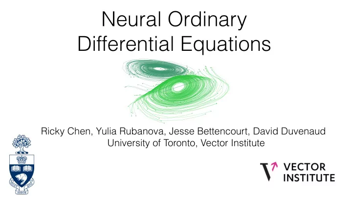
Neural Ordinary Differential Equations Ricky Chen, Yulia Rubanova, Jesse Bettencourt, David Duvenaud University of Toronto, Vector Institute

Background: ODE Solvers • Vector-valued z changes in time • Time-derivative: z • Initial-value problem: given , find: + • Euler approximates with small steps: t z ( t + h ) = z ( t ) + hf ( z , t )

Resnets as Euler integrators 5 def f(z, t, θ ): return nnet(z, θ [t]) 4 def resnet(z): 3 for t in [1:T]: Depth z = z + f(z, t, θ ) 2 return z 1 0 5 0 5 Input/Hidden/Output z

Related Work • Continuous-time nets once seemed natural 
 LeCun (1988), Pearlmutter (1995) • Solver-inspired architectures: 
 Lu et al. (2017), Haber & Ruthotto (2017), 
 Ruthotto & Haber (2018) • ODE-inspired training methods: 
 Chang et al. (2017, 2018)

5 4 def f(z, t, θ ): return nnet(z, θ [t]) 3 Depth def resnet(z, θ ): for t in [1:T]: 2 z = z + f(z, t, θ ) return z 1 0 5 0 5 z Input/Hidden/Output

5 4 def f(z, t, θ ): 
 return nnet([z, t], θ ) 3 Depth def resnet(z, θ ): for t in [1:T]: 2 z = z + f(z, t, θ ) return z 1 0 5 0 5 z Input/Hidden/Output

5 4 def f(z, t, θ ): 
 return nnet([z, t], θ ) 3 Depth def resnet(z, θ ): for t in [1:T]: 2 z = z + f(z, t, θ ) return z 1 0 5 0 5 z Input/Hidden/Output

5 t = 1 4 def f(z, t, θ ): 
 return nnet([z, t], θ ) 3 Depth def ODEnet(z, θ ): return ODESolve(f, z, 0, 1, θ ) 2 1 t = 0 0 5 0 5 z Input/Hidden/Output z

How to train an ODE net? L ( θ ) ∂ L ∂ θ = ? • Don’t backprop through solver: High memory cost, extra numerical error • Approximate the derivative, don’t differentiate the approximation!

Continuous-time Backpropagation Adjoint sensitivities: 
 Standard Backprop: • Can build adjoint dynamics with (Pontryagin et al., 1962): autodiff, compute all gradients with a ( t ) = ∂ L another ODE solve: 
 ∂ z ( t ) def f_and_a([z, a, d], t): ∂ f ( z t , θ ) ∂ z t ∂ L = a ( t ) ∂ f ( z t , t , θ ) ∂ a ( t ) return [f, -a*df/da, -a*df/d θ ) = ∂ z t +1 ∂ z t +1 ∂ z t ∂ t ∂ z [z0, dL/dx, dL/d θ ] = ∂ θ = ∫ t 0 ODESolve(f_and_a, 
 ∂ f ( z t , θ ) ∂ L = ∂ L ∂ L a ( t ) ∂ f ( z ( t ), t , θ ) dt [z(t1), dL/dz(t), 0], t1, t0) ∂ θ t ∂ θ t ∂ z t ∂ θ t 1

O(1) Memory Gradients • No need to store activations, just run dynamics backwards from State output. Adjoint State • Reversible ResNets (Gomez et al., 2018) must partition dimensions.

Drop-in replacement for Resnets 7x7 conv, 64, /2 pool, /2 • Same performance with fewer parameters. 3x3 conv, 64 3x3 conv, 64 30 layers 3x3 conv, 512 3x3 conv, 512 avg pool fc 1000

How deep are ODE-nets? • ‘Depth’ is left to ODE solver. • Dynamics become more demanding during training Num 
 evals • 2-4x the depth of resnet architectures • Chang et al. (2018) build such a schedule by hand Training Epoch

Explicit Error Control ODESolve(f, x, t0, t1, θ , tolerance) Numerical 
 error Number of dynamics evaluations

Reverse vs Forward Cost • Empirically, reverse pass roughly half as expensive as forward pass • Again, adapts to instance difficulty • Num evaluations comparable to number of layers in modern nets

Speed-Accuracy Tradeoff output = ODESolve(f, z0, t0, t1, theta, tolerance) • Time cost is dominated by evaluation of dynamics tolerance • Roughly linear with number of forward evaluations

Continuous-time models ODE Solve( z t 0 , f, θ f , t 0 , ..., t N ) • Well-defined state at all times z t 1 z t 0 z t N z t i • Dynamics separate from inference • Irregularly-timed observations. ˆ ˆ ˆ ˆ x t 0 x t 1 x t i x t N

Continuous-time RNNs • Can do VAE-style inference with an RNN encoder • Actually, more like a Deep Kalman Filter ODE Solve( z t 0 , f, θ f , t 0 , ..., t M ) RNN encoder q ( z t 0 | x t 0 ...x t N ) z t 1 z t N +1 h t 1 h t N z t M z t 0 z t N µ ~ … σ Latent space Data space x ( t ) ˆ x ( t ) t N +1 t M t N +1 t N t 0 t 1 t N t M t t 1 Observed Unobserved Prediction Extrapolation

Continuous-time models Recurrent Neural Net Latent ODE

Latent space interpolation Each latent point corresponds to a trajectory

Poisson Process Likelihoods • Can condition on arrival times inferred 
 to inform latent state rate Time

Instantaneous 
 Change of variables Change of Variables • Worst-case cost O(D^2). • Worst-case cost O(D^3). • Only need continuously • Requires invertible f differentiable f

Continuous Normalizing Flows • Reversible dynamics, so can train from data by maximum likelihood • No discriminator or recognition network, train by SGD • No need to partition dimensions

Trading Depth for Width