Differential Equations Classification and Simulation November 25, - PDF document

Differential Equations Classification and Simulation November 25, 2008 M. Emmerich, LIACS 1

Classification • Ordinary Differential Equations • Systems of Coupled Ordinary Differential Equations • Partial Differential Equations 2

Ordinary differential equations • Consider the equation: dh dt = Q ( t ) /A ( h ) (1) • Here h ( t ) describes the height of a fluid in a reservoir depending on time, Q ( t ) describes the inflow in m 3 /s , and A ( h ) describes the area of the reservoir, which depends on the height. • The equation describes an ordinary differ- ential equation (ODE) • In this lecture we will review methods to solve ODEs numerically 3

Ordinary differential equation (2) • An ordinary differential equation is an equa- tion that involves one or more derivatives of an unknown function • A solution of an differential equation is a specific function that satisfies the equa- tion, e.g. Equation Solution x ′ = x x ( t ) = c e t x ′ = a x ( t ) = at + c x ′′ + 9 x = 0 x ( t ) c 1 sin(3 t ) + c 2 cos(3 t ) • the letter c dentes an arbitrary constant • this indicates that, in general, ODEs have not a unique solution function 4

Initial-value problem • Given an initial value x ( t 0 ) at some point t 0 the solution curve of the ODE gets unique, e.g. x ′ = Equation: x ce t Solution: x ( t ) = Initial-value: x (2) = 5 5 e 2 e t Solution: x ( t ) = • ODE problems with an initial value given will be called initial-value problems • Given the initial value, all past and future states of the system described as ODE are determined 5

Boundary value problem − ( y ′ ) 2 − 2 by + 2 yy ′′ = 0 y (0) = a 0 , y (1) = a 1 • Due to the type of condition, the problem is a so-called boundary value problem • The differential equation is of 2nd order, as it includes first and second derivatives • So-called shooting methods are used for the numerical solutions of boundary value problems for ODEs 6

Solution of ODE • Analytically, e.g. dV/dt = at + b ⇔ (2) dV = ( at + b ) dt ⇔ (3) � � dV = ( at + b ) dt (4) a 2 t 2 + bt + C V ( t ) = (5) • Symbolic solvers (Maple, DeRive, Mathe- matica) ode := D(x)(t) = 2 t + 4; dsolve({ode, x(2)=5},x(t)); • Numerically (Euler, Runge-Kutta) 7

Coupled Differential Equations • Example are Lotka Volterra Equations de- scribing a predator prey system: x ′ = (6) ayx − b y ′ = − cyx + d (7) x is the population size of predator y is the population size of prey a : birth rate of predator (depends on y ) b : death rate of predator c : death rate of prey (depends on x ) d : birth rate of prey • The system results in two solution curves 8

Other examples of Coupled ODE • chemical reaction systems state variables: concentrations of compo- nents constants:kinetic constants • environmental models state variables: CO 2 , temperature constant: energy intake from sun, heat absorption rates • market models state variables: price and demand constant: available ressources 10

Partial derivatives • Consider a landscape described by the graph of function f ( x 1 , x 2 ) ∂f • ∂x 1 denotes the slope of the landscape in � 1 � direction 0 ∂f • ∂x 2 denotes the slope of the landscape in � 0 � direction 1 • for d -dimensional function f ( x 1 , . . . , x d ), ∂f ( x ) ∂x i denotes the slope of the landscape in the direction of the i − th unit vector � e i • for differentiable functions f : ∂f ( x ) f ( � x 0 ) + f ( � x 0 + h� e i ) ( � x 0 ) = lim (8) ∂x i h h → 0 11

Gradient x ) = ( ∂f ∂x 1 , . . . , ∂f • grad f ( � ∂x d ) is the gradient of f at � x • The gradient points in the direction of steep- est ascent of f ( � x ) • The length of the gradient depends on the steepness in that direction 12

Partial differential equations • A partial differential equation is an equa- tion with partial derivatives and typically also a derivative in time • A very simple example: ( ∂f ∂x, ∂f ∂y, ∂f ∂t ) T = grad f = ( s x , s y , s t ) T (9) • Solution of this equation is a moving plane: f ( x, y, t ) = s x · x + s y y + s t t + c (10) • It has a well defined solution, if we provide a condition f ( x 0 , y 0 , t 0 ) = h 0 13

Partial differential equations • Partial differential equations can also be defined on vector fields • Navier Stokes Equation for fluid flow of compressible fluids are important example • A closed form solution of these equations is one of the millenium problems in math- ematics • However, we can look at special cases, e.g. incompressible fluids • Or, we can solve the equations numeri- cally using finite difference or finite ele- ments methods ∗ ∗ in turbulent regime difficulties will arise, however 14

Wave equation with u being the displacement of a particle: ∂ 2 u ∂x 2 + ∂ 2 u ∂y 2 + ∂ 2 u ∂z 2 − ∂ 2 u ∂t 2 = 0 Heat equation with u being the local temper- ature: ∂ 2 u ∂x 2 + ∂ 2 u ∂y 2 + ∂ u ∂z 2 − ∂u ∂z = 0 Laplace’s equation, where u represents the ve- locity potential of a incompressible and irrotat- able fluid: ∂ 2 u ∂x 2 + ∂ 2 u ∂y 2 + ∂ 2 u ∂z 2 = 0 15

Numerical solution of ODE • Taylor methods can approximate a solution to a differentiable function • Differentiable functions can be locally ap- proximated by the Taylor series x ( t + h ) = x ( t )+ hx ′ ( t )+ h 2 2 x ′′ ( t )+ . . . + h n n ! h n x ( n ) ( t ) • when only terms up to order n are consid- ered the method is called a Taylor method of order n 16

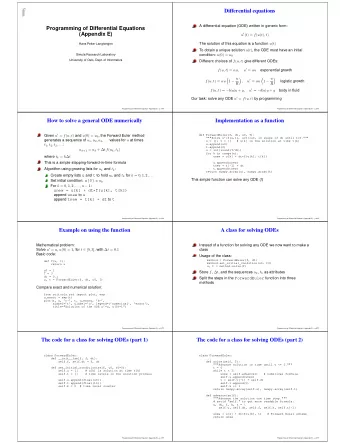
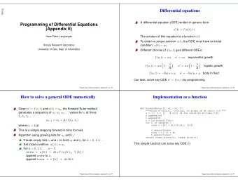
Euler’s method • The Taylor method of order 1 is called the Euler method • To find an approximate solution to the ini- tial value problem x ′ = f ( t, x ( t )) , x ( a ) = x a (11) over the interval [ a, b ], the first two terms of the Taylor series are used: x ( t + h ) = x ( t ) + hf ( t, x ( t )) (12) • Formally this process is an iterated func- tion system, and we could compute its Ljapunov coefficient 17

Pseudo code of Euler method • The following pseudocode produces an ap- proximation of the solution trajectory over the interval [ a, b ] with n points Euler method input: n, a, b, x a h ← ( b − a ) /n t ← a print 0 , t, x for all k ∈ (1 , . . . , n ) do x ← x + hf ( t, x ) t ← t + h print k, t, x end for • Eulers method is not very accurate. The truncation error is O ( h 2 ) in one iteration, i.e. if we decrease h the error will decrease at a rate proportional to h 2 18

Taylor method of order n • Given x ′ we first have to determine deriva- tive functions x ′′ , . . . , x ( n ) • Then we can use the following algorithm to determine approximation over interval [ a, b ] Taylor method of order n input: a, b, x a , n h ← ( b − a ) /n t ← a print 0,t,x for all k ∈ (1 , . . . , n ) do x ← x + hx ′ + h 2 2 x ′′ + . . . + h n n ! x ( n ) t → t + kh print k, t, x end for 19

Accuracy of Taylor method • How many digits of the approximation are reliable? • Coarse assessment of the error for n = 4: • The first term not included in Taylor series is 1 5! h 5 x (5) ( t ) 100 the value of h 5 is 1 • For example, if h = 10 10 and depending on the order of mag- nitude of x (5) we can assess the error. 20

• Two types of errors are to be considered here: – Local truncation error: Error we make when computing x ( t + h ) from x ( t ), this 5! h 5 x (5) or, in general, 1 is estimated by order O ( h n ) – The second type of error is the cumu- lated effect of the iteration ( x ( t ) is al- ready wrong, for t > a )

Roundoff error • In addition the roundoff error has to be considered • In one iteration roundoff errors are typically small, but accumulated over several itera- tions their impact can grow • Interval arithmetics can be used to round- off error 21

Interval arithmetics • Some rules of interval arithmetics, e.g. for a, b, c, d > 0: [ a, b ] + [ c, d ] = [ a + c, b + d ] (13) [ a, b ] + [ c, d ] = [ a − d, b − c ] (14) [ a, b ] ∗ [ c, d ] = [ a ∗ c, b ∗ d ] (15) [ a, b ] / [ c, d ] = [ a/d, b/d ] (16) • For bounding the result of the error f ([ a, b ]) the inclusion function can be derived with f ([ a, b ]) = [min { f ( x ) | x ∈ [ a, b ] } , max { f ( x ) | x ∈ [ a, b ] } ] • Roundoff errors are particular harmful in iterated systems with high Ljapunov coef- ficient 22

Runge Kutta method • Runge Kutta methods ∗ imitate the Taylor method of order n without needing an ex- plicit formula for higher order derivatives • Order 4 Runge Kutta method reads: x ( t + h ) = x ( t ) + 1 6( F 1 + 2 F 2 + 2 F 3 + F 4 ) where F 1 = hf ( t, x ) (17) hf ( t + 1 2 h, x + 1 F 2 = 2 F 1 ) (18) hf ( t + 1 2 h, x + 1 = 2 F 2 ) (19) F 3 = hf ( t + h, x + F 3 ) (20) F 4 • the next iterate is computed at the expense of computing f four times ∗ Carl Runge and William Kutta 23

Runge Kutta Method (2) • The error of the order-4 Runge Kutta method is of order O ( h 4 ), as opposed to the order- 4 Taylor method with error of order O ( h 5 ) • In practical situations a tolerance is pre- scribed and the method must not produce an error beyond this tolerance • The adaptive Runge Kutta Fehlberg method adapts the stepsize h to reach the desired accuracy • The allowable step-size is estimated in each step • Depending on whether the bound is met the step-size is either increased or decreased 24