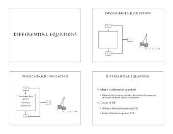
Differential equations Programming of Differential Equations A - PDF document

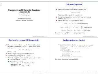
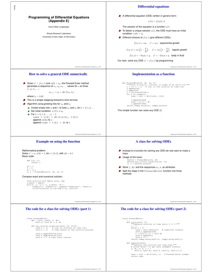
5mm. Differential equations Programming of Differential Equations A differential equation (ODE) written in generic form: (Appendix E) u ′ ( t ) = f ( u ( t ) , t ) Hans Petter Langtangen The solution of this equation is a function u ( t ) To obtain a unique solution u ( t ) , the ODE must have an initial Simula Research Laboratory condition: u (0) = u 0 University of Oslo, Dept. of Informatics Different choices of f ( u, t ) give different ODEs: u ′ = αu f ( u, t ) = αu, exponential growth 1 − u 1 − u � � u ′ = αu � � f ( u, t ) = αu , logistic growth R R u ′ = − b | u | u + g f ( u, t ) = − b | u | u + g, body in fluid Our task: solve any ODE u ′ = f ( u, t ) by programming Programming of Differential Equations (Appendix E) – p.1/ ?? Programming of Differential Equations (Appendix E) – p.2/ ?? How to solve a general ODE numerically Implementation as a function Given u ′ = f ( u, t ) and u (0) = u 0 , the Forward Euler method def ForwardEuler(f, dt, u0, T): """Solve u’=f(u,t), u(0)=u0, in steps of dt until t=T.""" generates a sequence of u 1 , u 2 , u 3 , . . . values for u at times u = []; t = [] # u[k] is the solution at time t[k] u.append(u0) t 1 , t 2 , t 3 , . . . : t.append(0) u k +1 = u k + ∆ t f ( u k , t k ) n = int(round(T/dt)) for k in range(n): unew = u[k] + dt*f(u[k], t[k]) where t k = k ∆ t u.append(unew) This is a simple stepping-forward-in-time formula tnew = t[-1] + dt t.append(tnew) Algorithm using growing lists for u k and t k : return numpy.array(u), numpy.array(t) Create empty lists u and t to hold u k and t k for k = 0 , 1 , 2 , . . . Set initial condition: u[0] = u 0 This simple function can solve any ODE (!) For k = 0 , 1 , 2 , . . . , n − 1 : unew = u[k] + dt*f(u[k], t[k]) append unew to u append tnew = t[k] + dt to t Programming of Differential Equations (Appendix E) – p.3/ ?? Programming of Differential Equations (Appendix E) – p.4/ ?? Example on using the function A class for solving ODEs Mathematical problem: Instead of a function for solving any ODE we now want to make a Solve u ′ = u , u (0) = 1 , for t ∈ [0 , 3] , with ∆ t = 0 . 1 class Basic code: Usage of the class: method = ForwardEuler(f, dt) def f(u, t): method.set_initial_condition(u0, t0) return u u, t = method.solve(T) u0 = 1 Store f , ∆ t , and the sequences u k , t k as attributes T = 3 dt = 0.1 Split the steps in the ForwardEuler function into three u, t = ForwardEuler(f, dt, u0, T) methods Compare exact and numerical solution: from scitools.std import plot, exp u_exact = exp(t) plot(t, u, ’r-’, t, u_exact, ’b-’, xlabel=’t’, ylabel=’u’, legend=(’numerical’, ’exact’), title="Solution of the ODE u’=u, u(0)=1") Programming of Differential Equations (Appendix E) – p.5/ ?? Programming of Differential Equations (Appendix E) – p.6/ ?? The code for a class for solving ODEs (part 1) The code for a class for solving ODEs (part 2) class ForwardEuler: class ForwardEuler: def __init__(self, f, dt): ... self.f, self.dt = f, dt def solve(self, T): """Advance solution in time until t <= T.""" def set_initial_condition(self, u0, t0=0): t = 0 self.u = [] # u[k] is solution at time t[k] while t < T: self.t = [] # time levels in the solution process unew = self.advance() # numerical formula self.u.append(unew) self.u.append(float(u0)) t = self.t[-1] + self.dt self.t.append(float(t0)) self.t.append(t) self.k = 0 # time level counter self.k += 1 return numpy.array(self.u), numpy.array(self.t) def advance(self): """Advance the solution one time step.""" # avoid "self." to get more readable formula: u, dt, f, k, t = \ self.u, self.dt, self.f, self.k, self.t[-1] unew = u[k] + dt*f(u[k], t) # Forward Euler scheme return unew Programming of Differential Equations (Appendix E) – p.7/ ?? Programming of Differential Equations (Appendix E) – p.8/ ??

Verifying the class implementation Using a class to hold the right-hand side f ( u, t ) Mathematical problem: Mathematical problem: u ′ = 0 . 2 + ( u − h ( t )) 4 , � 1 − u ( t ) � u (0) = 3 , t ∈ [0 , 3] u ′ ( t ) = αu ( t ) u (0) = u 0 , t ∈ [0 , 40] , R u ( t ) = h ( t ) = 0 . 2 t + 3 (exact solution) Class for right-hand side f ( u, t ) : The Forward Euler method will reproduce such a linear u exactly! Code: class Logistic: def __init__(self, alpha, R, u0): self.alpha, self.R, self.u0 = alpha, float(R), u0 def f(u, t): return 0.2 + (u - h(t))**4 def __call__(self, u, t): # f(u,t) return self.alpha*u*(1 - u/self.R) def h(t): return 0.2*t + 3 Main program: u0 = 3; dt = 0.4; T = 3 method = ForwardEuler(f, dt) problem = Logistic(0.2, 1, 0.1) method.set_initial_condition(u0, 0) T = 40; dt = 0.1 u, t = method.solve(T) method = ForwardEuler(problem, dt) u_exact = h(t) method.set_initial_condition(problem.u0, 0) print ’Numerical: %s\nExact: %s’ % (u, u_exact) u, t = method.solve(T) Programming of Differential Equations (Appendix E) – p.9/ ?? Programming of Differential Equations (Appendix E) – p.10/ ?? Figure of the solution Ordinary differential equations Mathematical problem: Logistic growth: alpha=0.2, dt=0.1, 400 steps 1 u ′ ( t ) = f ( u, t ) 0.9 Initial condition: 0.8 u (0) = u 0 0.7 Possible applications: 0.6 u 0.5 Exponential growth of money or populations: f ( u, t ) = αu , α = const 0.4 Logistic growth of a population under limited resources: 0.3 0.2 1 − u � � f ( u, t ) = αu R 0.1 0 5 10 15 20 25 30 35 40 t where R is the maximum possible value of u Radioactive decay of a substance: f ( u, t ) = − αu , α = const Programming of Differential Equations (Appendix E) – p.11/ ?? Programming of Differential Equations (Appendix E) – p.12/ ?? Numerical solution of ordinary differential equations A superclass for ODE methods Numerous methods for u ′ ( t ) = f ( u, t ) , u (0) = u 0 Common tasks for ODE solvers: The Forward Euler method: Store the solution u k and the corresponding time levels t k , k = 0 , 1 , 2 , . . . , N u k +1 = u k + ∆ t f ( u k , t k ) Store the right-hand side function f ( u, t ) The 4th-order Runge-Kutta method: Store the time step ∆ t and last time step number k Set the initial condition u k +1 = u k + 1 6 ( K 1 + 2 K 2 + 2 K 3 + K 4 ) Implement the loop over all time steps Code for the steps above are common to all classes and hence placed in superclass ODESolver K 1 = ∆ t f ( u k , t k ) , ∆ t f ( u k + 1 2 K 1 , t k + 1 Subclasses, e.g., ForwardEuler , just implement the specific = 2∆ t ) , K 2 stepping formula in a method advance ∆ t f ( u k + 1 2 K 2 , t k + 1 K 3 = 2∆ t ) , K 4 = ∆ t f ( u k + K 3 , t k + ∆ t ) There is a jungle of different methods – how to program? Programming of Differential Equations (Appendix E) – p.13/ ?? Programming of Differential Equations (Appendix E) – p.14/ ?? The superclass code Implementation of the Forward Euler method class ODESolver: Subclass code: def __init__(self, f, dt): self.f = f class ForwardEuler(ODESolver): self.dt = dt def advance(self): u, dt, f, k, t = \ def set_initial_condition(self, u0, t0=0): self.u, self.dt, self.f, self.k, self.t[-1] self.u = [] # u[k] is solution at time t[k] self.t = [] # time levels in the solution process unew = u[k] + dt*f(u[k], t) self.u.append(u0) return unew self.t.append(t0) self.k = 0 # time level counter Application code for u ′ = u , u (0) = 1 , t ∈ [0 , 3] , ∆ t = 0 . 1 : def solve(self, T): t = 0 from ODESolver import ForwardEuler while t < T: def test1(u, t): unew = self.advance() # the numerical formula return u self.u.append(unew) method = ForwardEuler(test1, dt=0.1) t = self.t[-1] + self.dt method.set_initial_condition(u0=1) self.t.append(t) u, t = method.solve(T=3) self.k += 1 plot(t, u) return numpy.array(self.u), numpy.array(self.t) def advance(self): raise NotImplementedError Programming of Differential Equations (Appendix E) – p.15/ ?? Programming of Differential Equations (Appendix E) – p.16/ ??