Population Modeling with Ordinary Differential Equations Michael J. - PDF document

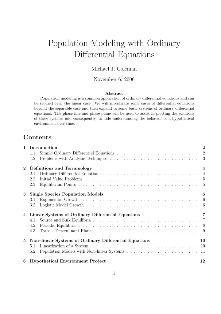
Population Modeling with Ordinary Differential Equations Michael J. Coleman November 6, 2006 Abstract Population modeling is a common application of ordinary differential equations and can be studied even the linear case. We will investigate some cases of differential equations beyond the separable case and then expand to some basic systems of ordinary differential equations. The phase line and phase plane will be used to assist in plotting the solutions of these systems and consequently, to aide understanding the behavior of a hypothetical environment over time. Contents 1 Introduction 2 1.1 Simple Ordinary Differential Equations . . . . . . . . . . . . . . . . . . . . . . . . 2 1.2 Problems with Analytic Techniques . . . . . . . . . . . . . . . . . . . . . . . . . . 3 2 Definitions and Terminology 4 2.1 Ordinary Differential Equation . . . . . . . . . . . . . . . . . . . . . . . . . . . . . 4 2.2 Initial Value Problems . . . . . . . . . . . . . . . . . . . . . . . . . . . . . . . . . 5 2.3 Equilibrium Points . . . . . . . . . . . . . . . . . . . . . . . . . . . . . . . . . . . 5 3 Single Species Population Models 6 3.1 Exponential Growth . . . . . . . . . . . . . . . . . . . . . . . . . . . . . . . . . . 6 3.2 Logistic Model Growth . . . . . . . . . . . . . . . . . . . . . . . . . . . . . . . . . 6 4 Linear Systems of Ordinary Differential Equations 7 4.1 Source and Sink Equilibria . . . . . . . . . . . . . . . . . . . . . . . . . . . . . . . 7 4.2 Periodic Equilibria . . . . . . . . . . . . . . . . . . . . . . . . . . . . . . . . . . . 8 4.3 Trace – Determinant Plane . . . . . . . . . . . . . . . . . . . . . . . . . . . . . . . 9 5 Non–linear Systems of Ordinary Differential Equations 10 5.1 Linearization of a System . . . . . . . . . . . . . . . . . . . . . . . . . . . . . . . 10 5.2 Population Models with Non–linear Systems . . . . . . . . . . . . . . . . . . . . . 11 6 Hypothetical Environment Project 12 1

1 Introduction 1.1 Simple Ordinary Differential Equations The simplest type of differential equation is the standard case you find in calculus • Completely non–autonomous differential equations. These are nothing more than some of those MATH–032 integrals. Example: dx dt = t 2 + t Solution: t 3 + t 2 � � t 2 + t � x ( t ) = dt = + C. 3 2 • Separable differential equations are types that you’ve probably encountered before and are not too hard to work out. Example: dx dt = ( x + 1) t Solution: Separate variables and integrate both sides with respect to the given variable. � � dx x + 1 = t dt Then we can integrate these equations to obtain a general solution t 2 � = � x + 1 � � ln + C 2 2

1.2 Problems with Analytic Techniques There are many different examples that arise in differential equa- tions which raise problems with these analytic techniques. Here are just a couple. Example: The following differential equation is separable. [1] dx x dt = x + 1 Solution: We can separate and integrate easily as follows. � � 1 � � x + x dx = dt Problem: There is no way to algebraically solve the equation � + x 2 � x � � ln = t + C. 2 Example: This is a perfectly separable differential equation. [1] dx dt = sec( x 2 ) Problem: It’s a pity the left hand integration is perhaps impossible. � � cos( x 2 ) dx = dt 3

2 Definitions and Terminology 2.1 Ordinary Differential Equation An ordinary differential equation [2] relates the ordinary deriva- tives of an unknown function and possibly the function x ( t ) itself. It has the general form dt , d 2 x dt 2 , d 3 x � � t, x, dx = 0 . G dt 3 , . . . where the function G determines which derivatives are involved in the equations and the extent to which each is involved. Familiar differential equations, such as the following, take this form. Examples: t 2 + t − dx dt = 0 x + dx dt = 0 x 2 + x + d 4 x = 0 dt 4 Newton’s Law: One the most common differential equations used in physical application is Newton’s F = ma. Acceleration is the second derivative of a displacement function x ( t ) so, we have the differential equation F − m d 2 x = 0 . dt 2 4

2.2 Initial Value Problems • An initial value problem involves both a differential equation and a prescribed value for the unknown function x ( t ) at some initial time t 0 . Express such a problem as dt , d 2 x dt 2 , d 3 x � � t, x, dx F dt 3 , . . . = 0 with x ( t 0 ) = x 0 • A solution to an initial value problem must satisfy both the differen- tial equation as well as the initial value prescribed at the particular initial time t 0 . 2.3 Equilibrium Points An equilibrium point x ∗ is one where a solution of the differential equation remains fixed at x ∗ for all time. In other words x ( t ) = x ∗ for all t ∈ R . Equivalently, equilibrium points are determined by locating the points where dx = 0 . dt For a system of differential equations, we will have something like: dx dy dt = f ( x, y ) and dt = g ( x, y ) . In this instance, equilibrium points are all such points ( x ∗ , y ∗ ) which satisfy both f ( x, y ) = 0 and g ( x, y ) = 0 . 5

3 Single Species Population Models 3.1 Exponential Growth We just need one population variable in this case. The simplest (yet– incomplete model) is modeled by the rate of growth being equal to the size of the population. Exponential Growth Model: A differential equation of the separable class. dP = kP with P (0) = P 0 dt We can integrate this one to obtain � dP � P ( t ) = Ae kt = = dt ⇒ kP where A derives from the constant of integration and is calculated using the initial condition. This solution may be easier to see on a phase line. 3.2 Logistic Model Growth Exponential growth is not quite accurate since the environmental sup- port system for a given species is likely not infinite. Logistic Model: dP = kP ( M − P ) dt where M is some maximum population or what environmentalists might call the “carrying capacity”. We can better capture the behavior of a population model on a phase line and derivative field. 6

4 Linear Systems of Ordinary Differential Equations For linear systems, we consider the effects of two unknown functions on each other. A two by two system of linear ordinary differential equations has the form dx  � x � a b � x dt = ax + by � � � d  or = · y c d y dt dy dt = cx + dy  If we set Y to be the unknown vector and let A be the coefficient matrix, then we have a matrix equation d Y dt = AY . (1) 4.1 Source and Sink Equilibria Theorem: [1] If A has distinct real eigenvalues λ 1 and λ 2 with corre- sponding eigenvectors v 1 and v 2 , then the general solution of (1) is Y ( t ) = k 1 exp ( λ 1 t ) v 1 + k 2 exp ( λ 2 t ) v 2 . Example: An unstable system of differential equations � 1 0 � x � x � dx dt = x � � � d or = · dy dt = 2 y y 0 2 y dt The coefficient matrix A has λ + = 2 and λ − = 1 with eigenvectors v + = (0 , 1) and v − = (1 , 0). Then the general solution is � 1 � 0 � � + k 2 e 2 t Y ( t ) = k 1 e t . 0 1 7

4.2 Periodic Equilibria Theorem: [1] If the eigenvalues of the coefficient matrix A are complex (having the form λ = α ± iβ ), then the solution of (1) is Y ( t ) = e αt � � cos( βt ) + i sin( βt ) v where v is an eigenvector of A . Example: Periodic solutions. dx � x � 0 − 1 � x  dt = − y � � � d  or = · 1 0 y y dt dy dt = x  We get Char( A ) = λ 2 + 1 = 0. Hence λ = ± i . � i � Only one of the eigenvectors is necessary in this case. Take v = , 1 corresponding to λ = i and coming from � 0 − 1 � � v 1 � iv 1 � � Av = = = λ v 1 0 v 2 iv 2 So, the solution works out to be � � i � − sin( t ) + i cos( t ) � � � Y ( t ) = cos( t ) + i sin( t ) = 1 cos( t ) + i sin( t ) Then we have � cos( t ) � − sin( t ) � � Y ( t ) = + i = Y Re ( t ) + i Y Im ( t ) cos( t ) sin( t ) The real and imaginary parts are each independent solutions to the sys- tem of differential equations. 8

4.3 Trace – Determinant Plane One can essentially learn about the behavior of a linear system of the form � x � a b � x � � � d = · y c d y dt simply by knowing the eigenvalues of the coefficient matrix. These are encapsulated in the characteristic equation Char( A ) = λ 2 − Tr( A ) λ + Det( A ) = 0 . Let T denote the trace and D the determinant of the matrix so that we may write (more compactly) the discriminant of this quadratic: T 2 − 4 D. When this quantity is larger than 0, there exist two real roots (hence there are two real eigenvalues for the system). When this quantity is less than 0, there exist two complex roots (and hence there are two complex eigenvalues for the system). To better assess how differing values of D and T affect the eigenvalues, T 2 we plot the curve D = 4 in the plane and isolate regions of varying eigenvalue characteristics. 9