Neural Networks: Multi-Layer Networks & Back-Propagation M. - PowerPoint PPT Presentation

Neural Networks: Multi-Layer Networks & Back-Propagation M. Soleymani Artificial Intelligence Sharif University of Technology Spring 2019 Most slides have been adapted from Bhiksha Raj, 11-785, CMU 2019 and some from Fei Fei Li et. al, cs231n, Stanford 2017

Reasons to study neural computation • Neuroscience: To understand how the brain actually works. – Its very big and very complicated and made of stuff that dies when you poke it around. So we need to use computer simulations. • AI: To solve practical problems by using novel learning algorithms inspired by the brain – Learning algorithms can be very useful even if they are not how the brain actually works. 2

3

A typical cortical neuron • Gross physical structure: – There is one axon that branches – There is a dendritic tree that collects input from other neurons. • Axons typically contact dendritic trees at synapses – A spike of activity in the axon causes charge to be injected into the post-synaptic neuron. • Spike generation: – There is an axon hillock that generates outgoing spikes whenever enough charge has flowed in at synapses to depolarize the cell membrane. 4

� Binary threshold neurons • McCulloch-Pitts (1943): influenced Von Neumann. – First compute a weighted sum of the inputs. – send out a spike of activity if the weighted sum exceeds a threshold. – McCulloch and Pitts thought that each spike is like the truth value of a proposition and each neuron combines truth values to compute the truth value of another proposition! 𝑔 : Activation 𝑔 function 𝑗𝑜𝑞𝑣𝑢 & 𝑥 & 𝑥 ' 𝑗𝑜𝑞𝑣𝑢 ' 𝑔 * 𝑥 , 𝑦 , Σ , … 𝑥 ( 𝑗𝑜𝑞𝑣𝑢 ( 5

� A better figure 𝑦 & 𝑥 & 𝑥 ' 𝑦 ' z = * w 4 x 4 − 𝜄 𝑦 0 𝑥 0 + 4 ..... z = 81 if z ≥ 0 0 else 𝑦 ( 𝑥 ( 𝜄 • A threshold unit – “Fires” if the weighted sum of inputs and the “bias” T is positive 6

McCulloch-Pitts neuron: binary threshold binary McCulloch-Pitts neuron 𝑧 𝑦 & 𝑥 & 𝑥 ' 𝑦 ' 𝑧 𝜄 : activation threshold … 𝑥 ( 𝑧 = 81, 𝑨 ≥ 𝜄 𝑦 ( 0, 𝑨 < 𝜄 Equivalent to 1 𝑐 𝑦 & 𝑧 𝑥 & 𝑥 ' 𝑦 ' 𝑧 … 𝑥 ( bias: 𝑐 = −𝜄 𝑦 ( 7

Neural nets and the brain 𝑦 & 𝑥 & 𝑥 ' 𝑦 ' 𝑥 0 𝑦 0 + . .... 𝑦 ( 𝑥 ( −𝜄 • Neural nets are composed of networks of computational models of neurons called perceptrons 8

The perceptron 𝑦 & 𝑥 & 𝑥 ' 𝑦 ' 𝑥 0 𝑦 0 + . .... 1 if * 𝑥 , 𝑦 , ≥ 𝜄 y = , 0 else −𝜄 𝑦 ( 𝑥 ( • A threshold unit – “Fires” if the weighted sum of inputs exceeds a threshold – Electrical engineers will call this a threshold gate • A basic unit of Booleancircuits 9

� The “soft” perceptron (logistic) 𝒚 𝟐 𝒙 𝟐 𝒚 𝟑 𝒙 𝟑 z = * w 4 x 4 − θ 𝒚 𝟒 𝒙 𝟒 4 + ..... 1 y = 1 + exp(−z) 𝒚 𝑶 −𝜄 𝒙 𝑶 • A “squashing” function instead of a threshold at the output – The sigmoid “activation” replaces the threshold • Activation: The function that acts on the weighted combination of inputs (and threshold) 10

Sigmoid neurons • These give a real-valued output that is a smooth and bounded function of their total input. • Typically they use the logistic function – They have nice derivatives. 11

Other “activations” 𝒚 𝟐 𝒙 𝟐 sigmoid 𝒚 𝟑 𝒙 𝟑 1 1 𝒚 𝟒 𝒙 𝟒 1 + exp (−𝑨) + .... tanh 𝒄 𝒚 𝑶 𝒙 𝑶 tanh 𝑨 (1 + 𝑓 [ ) log • Does not always have to be a squashing function – We will hear more about activations later • We will continue to assume a “threshold” activation in this lecture 12

� Perceptron 𝑥 & 𝑦 & z = * w 4 x 4 + b 𝑦 ' 𝑥 ' 4 𝑦 0 𝑥 0 + .... 𝑦 ' 1 x 2 𝑐 𝑦 ( 𝑥 ( x 1 𝑦 & 0 • Lean this function – A step function across a hyperplane 13

� Learning the perceptron 𝑧 = b1 𝑗𝑔 * w 4 x 4 + b ≥ 0 𝑦 & 𝑥 & 4 𝑥 ' 𝑦 ' 0 𝑝𝑢ℎ𝑓𝑠𝑥𝑗𝑡𝑓 𝑦 0 𝑥 0 𝑦 ' + .... 𝑦 & 𝑦 ( 𝑐 𝑥 ( • Given a number of input output pairs, learn the weights and bias – Learn 𝑋 = [𝑥 & , … , 𝑥 ( ] and b, given several 𝑌, 𝑧 pairs 14

Restating the perceptron x 1 x 2 x 3 𝑋 ( x d W d+1 x d+1 =1 • Restating the perceptron equation by adding another dimension to 𝑌 (h& 𝑧 = 81 𝑗𝑔 ∑ 𝑥 , 𝑦 , ≥ 0 ,i& Where 𝑦 (h& = 1 0 𝑝𝑢ℎ𝑓𝑠𝑥𝑗𝑡𝑓 (h& • Note that the boundary ∑ 𝑥 , 𝑦 , ≥ 0 is now a hyperplane ,i& through origin 15

The Perceptron Problem (h& • Find the hyperplane that perfectly separates thetwo * 𝑥 , 𝑦 , = 0 groups of points ,i& 34 16

Perceptron Algorithm:Summary • Cycle through the traininginstances • Only update 𝒙 on misclassifiedinstances • If instance misclassified: – If instance is positive class 𝒙 = 𝒙 + 𝒚 – If instance is negative class 𝒙 = 𝒙 − 𝒚 17

A Simple Method: The Perceptron Algorithm 𝒙 +1 (blue) -1 (red) • Initialize: Randomly initialize the hyperplane – i.e. randomly initialize the normalvector 𝑥 • Classification rule 𝑡𝑗𝑕𝑜(𝒙 k 𝒚) – Vectors on the same side of the hyperplane as 𝑋 will be assigned +1 class, and those on the other side will be assigned -1 • The random initial plane will make mistakes 18

How to learn the weights: multi class example This example has been adopted from Hinton slides, “NN for Machine Learning”, coursera, 2015. 19

How to learn the weights: multi class example • If correct: no change • If wrong: – lower score of the wrong answer (by removing the input from the weight vector of the wrong answer) – raise score of the target (by adding the input to the weight vector of the target class) This example has been adopted from Hinton slides, “NN for Machine Learning”, coursera, 2015. 20

How to learn the weights: multi class example • If correct: no change • If wrong: – lower score of the wrong answer (by removing the input from the weight vector of the wrong answer) – raise score of the target (by adding the input to the weight vector of the target class) This example has been adopted from Hinton slides, “NN for Machine Learning”, coursera, 2015. 21

How to learn the weights: multi class example • If correct: no change • If wrong: – lower score of the wrong answer (by removing the input from the weight vector of the wrong answer) – raise score of the target (by adding the input to the weight vector of the target class) This example has been adopted from Hinton slides, “NN for Machine Learning”, coursera, 2015. 22

How to learn the weights: multi class example • If correct: no change • If wrong: – lower score of the wrong answer (by removing the input from the weight vector of the wrong answer) – raise score of the target (by adding the input to the weight vector of the target class) This example has been adopted from Hinton slides, “NN for Machine Learning”, coursera, 2015. 23

How to learn the weights: multi class example • If correct: no change • If wrong: – lower score of the wrong answer (by removing the input from the weight vector of the wrong answer) – raise score of the target (by adding the input to the weight vector of the target class) This example has been adopted from Hinton slides, “NN for Machine Learning”, coursera, 2015. 24

How to learn the weights: multi class example • If correct: no change • If wrong: – lower score of the wrong answer (by removing the input from the weight vector of the wrong answer) – raise score of the target (by adding the input to the weight vector of the target class) This example has been adopted from Hinton slides, “NN for Machine Learning”, coursera, 2015. 25

Single layer networks as template matching • Weights for each class as a template (or sometimes also called a prototype) for that class. – The winner is the most similar template. • The ways in which hand-written digits vary are much too complicated to be captured by simple template matches of whole shapes. • To capture all the allowable variations of a digit we need to learn the features that it is composed of. 26

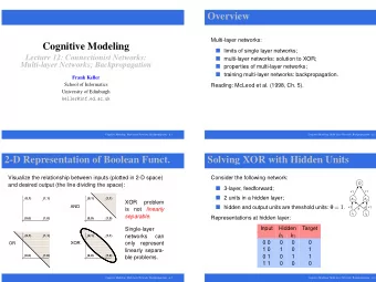
What binary threshold neurons cannot do • A binary threshold output unit cannot even tell if two single bit features are the same! • A geometric view of what binary threshold neurons cannot do • The positive and negative cases cannot be separated by a plane 27

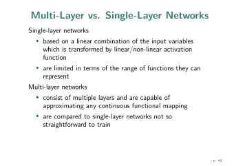
Networks with hidden units • Networks without hidden units are very limited in the input-output mappings they can learn to model. – More layers of linear units do not help. Its still linear. – Fixed output non-linearities are not enough. • We need multiple layers of adaptive, non-linear hidden units. But how can we train such nets? 28

The multi-layer perceptron • A network of perceptrons – Generally “layered ” 29

Feed-forward neural networks • Also called Multi-Layer Perceptron (MLP) 30