Neural networks and Reinforcement learning review CS 540 Yingyu - PowerPoint PPT Presentation
Neural networks and Reinforcement learning review CS 540 Yingyu Liang Neural Networks Outline Building unit: neuron Linear perceptron Non-linear perceptron The power/limit of a single perceptron Learning of a single
Neural networks and Reinforcement learning review CS 540 Yingyu Liang
Neural Networks
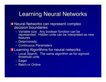
Outline • Building unit: neuron • Linear perceptron • Non-linear perceptron • The power/limit of a single perceptron • Learning of a single perceptron • Neural network: a network of neurons • Layers, hidden units • Learning of neural network: backpropagation (gradient descent)
Linear perceptron • Input: 𝑦 1 , 𝑦 2 , … , 𝑦 𝐸 (For notation simplicity, define 𝑦 0 = 1) • Weights: 𝑥 1 , 𝑥 2 , … , 𝑥 𝐸 • Bias: 𝑥 0 𝐸 • Output: 𝑏 = σ 𝑒=0 𝑥 𝑒 𝑦 𝑒 1 …
Nonlinear perceptron • Input: 𝑦 1 , 𝑦 2 , … , 𝑦 𝐸 (For notation simplicity, define 𝑦 0 = 1) • Weights: 𝑥 1 , 𝑥 2 , … , 𝑥 𝐸 • Bias: 𝑥 0 • Activation function: 𝑨 = step 𝑨 , sigmoid 𝑨 , relu 𝑨 , … 𝐸 • Output: 𝑏 = (σ 𝑒=0 𝑥 𝑒 𝑦 𝑒 ) 1 …
Example Question • Will you go to the festival? • Go only if Weather is favorable and at least one of the other two conditions is favorable ? Weather Company Proximity All inputs are binary; 1 is favorable
Multi-layer neural networks • Training: encode a label 𝑧 by an indicator vector ▪ class1=(1,0,0,…,0), class2=(0,1,0,…,0) etc. • Test: choose the class corresponding to the largest output unit (3) 𝑥 11 2 = (2) 𝑏 1 𝑦 𝑒 𝑥 1𝑒 (2) 2 𝑥 1𝑗 (3) 𝑥 11 𝑏 1 = 𝑏 𝑗 𝑒 (3) 𝑥 𝐿1 𝑗 𝑦 1 (2) 𝑥 21 (3) (2) 𝑥 12 … 𝑥 31 2 = (2) 𝑏 2 𝑦 𝑒 𝑥 2𝑒 (3) 𝑥 𝐿2 (2) 𝑥 12 𝑒 (2) 𝑥 22 𝑦 2 (3) 𝑥 13 2 𝑥 𝐿𝑗 (3) (2) 𝑏 𝐿 = 𝑏 𝑗 𝑥 32 2 = (2) 𝑏 3 𝑦 𝑒 𝑥 3𝑒 (3) 𝑥 𝐿3 𝑗 𝑒 slide 7
Learning in neural network • Again we will minimize the error ( 𝐿 outputs): 𝐿 𝐹 = 1 𝑧 − 𝑏 2 = 𝑏 𝑑 − 𝑧 𝑑 2 2 𝐹 𝑦 , 𝐹 𝑦 = 𝑦∈𝐸 𝑑=1 • 𝑦 : one training point in the training set 𝐸 • 𝑏 𝑑 : the 𝑑 -th output for the training point 𝑦 • 𝑧 𝑑 : the 𝑑 -th element of the label indicator vector for 𝑦 𝑏 1 1 𝑦 1 0 … = 𝑧 … 𝑦 2 0 𝑏 𝐿 0 slide 8
Backpropagation Layer (1) Layer (2) Layer (3) Layer (4) (4) 𝜀 1 (3) 𝑏 1 (4) 𝑥 11 𝑦 1 𝑏 1 𝑧 − 𝑏 2 = 𝐹 𝑦 𝑏 2 𝑦 2 4 𝑏 1 (3) 𝑥 11 (4) 𝑨 1 𝐹 𝑦 4 𝑏 2 (3) 𝑥 12 (4) = 𝜖𝐹 𝒚 (4) 𝜀 1 (4) = 2(𝑏 1 − 𝑧 1 )′ 𝑨 1 𝜖𝑨 1 𝜖𝐹 𝒚 (4) 𝑏 1 (3) (4) = 𝜀 1 By Chain Rule: 𝜖𝑥 11 slide 9
Backpropagation of 𝜀 Layer (1) Layer (2) Layer (3) Layer (4) (3) (4) (2) 𝜀 1 𝜀 1 𝜀 1 𝑦 1 𝑏 1 𝑧 − 𝑏 2 = 𝐹 𝑦 𝑏 2 𝑦 2 (3) (4) (2) 𝜀 2 𝜀 2 𝜀 2 Thus, for any neuron in the network: (𝑚) = 𝑚+1 𝑥 𝑙𝑘 𝑚+1 𝑚 𝜀 𝜀 𝑙 ′ 𝑨 𝑘 𝑘 𝑙 (𝑚) : 𝜀 of 𝑘 𝑢ℎ Neuron in Layer 𝑚 𝜀 𝑘 (𝑚+1) : 𝜀 of 𝑙 𝑢ℎ Neuron in Layer 𝑚 + 1 𝜀 𝑙 : derivative of 𝑘 𝑢ℎ Neuron in Layer 𝑚 w.r.t. its linear combination input 𝑚 ′ 𝑨 𝑘 (𝑚+1) : Weight from 𝑘 𝑢ℎ Neuron in Layer 𝑚 to 𝑙 𝑢ℎ Neuron in Layer 𝑚 + 1 slide 10 𝑥 𝑙𝑘
Example Question
Example Question
Example Question
Example Question
Convolution: discrete version • Given array 𝑣 𝑢 and 𝑥 𝑢 , their convolution is a function 𝑡 𝑢 +∞ 𝑡 𝑢 = 𝑣 𝑏 𝑥 𝑢−𝑏 𝑏=−∞ • Written as 𝑡 = 𝑣 ∗ 𝑥 or 𝑡 𝑢 = 𝑣 ∗ 𝑥 𝑢 • When 𝑣 𝑢 or 𝑥 𝑢 is not defined, assumed to be 0
Convolution illustration 𝑥 = [z, y, x] 𝑡 3 𝑣 = [a, b, c, d, e, f] xb+yc+zd 𝐱 𝟑 𝐱 𝟐 𝐱 𝟏 x y z 𝐯 𝟐 𝒗 𝟑 𝐯 𝟒 a b c d e f
Pooling illustration 𝑣 = [a, b, c, d, e, f] Max(b,c,d) 𝐯 𝟐 𝒗 𝟑 𝐯 𝟒 a b c d e f
Example question 𝑥 = [-1,1,1] What is the value 𝑡 = 𝑣 ∗ 𝑥 ? (Valid padding) 𝑣 = [1,2,3,4,5,6] 𝐱 𝟑 𝐱 𝟐 𝐱 𝟏 1 1 -1 1 2 3 4 5 6
Reinforcement Learning
Outline • The reinforcement learning task • Markov decision process • Value functions • Value iteration • Q functions • Q learning
Reinforcement learning as a Markov decision process (MDP) • Markov assumption agent = ( | , , , ,...) ( | , ) P s s a s a P s s a + − − + t 1 t t t 1 t 1 t 1 t t action state reward • also assume reward is Markovian environment = ( | , , , ,...) ( | , ) P r s a s a P r s a + − − + 1 1 1 1 t t t t t t t t a 0 a 1 a 2 s 0 s 1 s 2 r 0 r 1 r 2 Goal: learn a policy π : S → A for choosing actions that maximizes + + + 2 [ ...] where 0 1 E r r r + + 1 2 t t t 21 for every possible starting state s 0
Value function for a policy • given a policy π : S → A define = t ( ) [ ] assuming action sequence chosen V s E r t according to π starting at state s = 0 t we want the optimal policy π * where • p * = argmax p V p ( s ) for all s we’ll denote the value function for this optimal policy as V * ( s ) 22
Value iteration for learning V * ( s ) initialize V ( s ) arbitrarily loop until policy good enough { loop for s ∈ S { loop for a ∈ A { + ( , ) ( , ) ( ' | , ) ( ' ) Q s a r s a P s s a V s ' s S } ( ) max ( , ) V s Q s a a } } 23
Q function define a new function, closely related to V* + * ( , ) ( , ) ( ' ) Q s a E r s a E V s ' | , s s a if agent knows Q ( s, a ) , it can choose optimal action without knowing P ( s’ | s , a ) * * ( ) arg max ( , ) ( ) max ( , ) s Q s a V s Q s a a a and it can learn Q ( s, a ) without knowing P ( s ’ | s , a ) 24
Q learning for deterministic worlds ˆ for each s, a initialize table entry ( , ) 0 Q s a observe current state s do forever select an action a and execute it receive immediate reward r observe the new state s ’ update table entry ˆ ˆ + ( , ) max ( ' , ' ) Q s a r Q s a s ← s ’ ' a 25
Example question
Example question
Recommend
More recommend
Explore More Topics
Stay informed with curated content and fresh updates.
