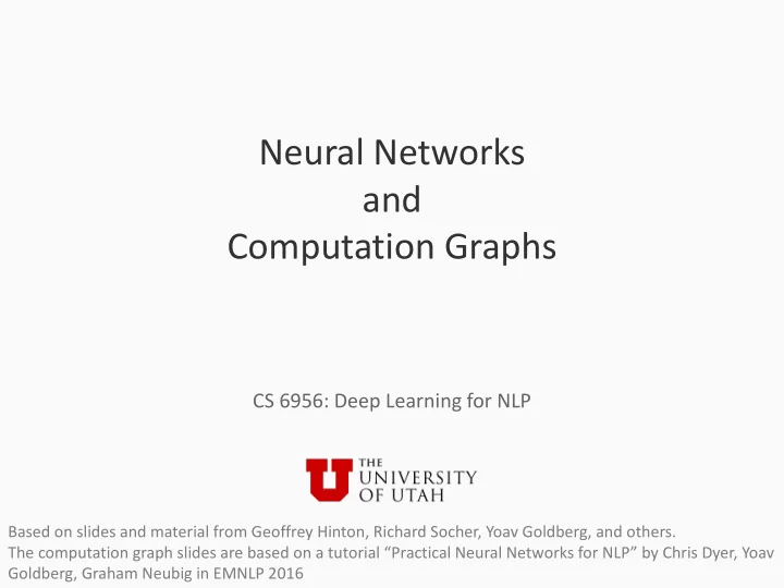
Neural Networks and Computation Graphs CS 6956: Deep Learning for - PowerPoint PPT Presentation

Let’s see some functions as graphs 𝐲 Y 𝐁𝐲 Expression Graph f 𝐍, 𝐰 = 𝐍𝐰 f 𝐕, 𝐖 = 𝐕𝐖 f 𝐯 = 𝐯 𝐔 𝐁 𝐲 32

Let’s see some functions as graphs 𝐲 Y 𝐁𝐲 Expression Graph f 𝐍, 𝐰 = 𝐍𝐰 f 𝐯, 𝐍 = 𝐯 𝐔 𝐍𝐯 f 𝐕, 𝐖 = 𝐕𝐖 𝐲 𝐁 f 𝐯 = 𝐯 𝐔 𝐁 We could have written the same function with a different graph. 𝐲 Computation graphs are not necessarily unique for a function 33

Let’s see some functions as graphs 𝐲 Y 𝐁𝐲 Expression Remember: The nodes also know how to compute derivatives with respect to each parent Graph f 𝐯, 𝐍 = 𝐯 𝐔 𝐍𝐯 𝐲 𝐁 34

Let’s see some functions as graphs 𝐲 Y 𝐁𝐲 Expression Remember: The nodes also know how to compute derivatives with respect to each parent Graph f 𝐯, 𝐍 = 𝐯 𝐔 𝐍𝐯 Derivative with respect to this 𝐲 𝐁 parent 𝜖𝑔 𝜖𝐯 = 𝐍 Y + 𝐍 𝐯 35

Let’s see some functions as graphs 𝐲 Y 𝐁𝐲 Expression Remember: The nodes also know how to compute derivatives with respect to each parent Graph f 𝐯, 𝐍 = 𝐯 𝐔 𝐍𝐯 Derivative with respect to this 𝐲 𝐁 parent 𝜖𝑔 𝜖𝐍 = 𝐯𝐯 ' 36

Let’s see some functions as graphs 𝐲 Y 𝐁𝐲 Expression Remember: The nodes also know 𝜖𝑔 𝜖𝑔 𝜖𝐲 = 𝐁 Y + 𝐁 𝐲 𝜖𝐁 = 𝐲𝐲 ' how to compute derivatives with respect to each parent Graph Together, we can compute derivatives of any function with f 𝐯, 𝐍 = 𝐯 𝐔 𝐍𝐯 respect to all its inputs, for any value of the input 𝐲 𝐁 𝜖𝑔 𝜖𝑔 𝜖𝐯 = 𝐍 Y + 𝐍 𝐯 𝜖𝐍 = 𝐯𝐯 ' 37

� Let’s see some functions as graphs 𝐲 Y 𝐁𝐲 + 𝐜 Y 𝐲 + 𝐝 Expression f 𝑦 L , 𝑦 K , 𝑦 g = h 𝑦 / 𝒋 Graph f 𝐍, 𝐰 = 𝐍𝐰 f 𝐕, 𝐖 = 𝐕𝐖 f 𝐯, 𝐰 = 𝐯 𝐔 𝐰 𝐝 f 𝐯 = 𝐯 𝐔 𝐁 𝐜 𝐲 38

� Let’s see some functions as graphs 𝑧 = 𝐲 Y 𝐁𝐲 + 𝐜 Y 𝐲 + 𝐝 Expression f 𝑦 L , 𝑦 K , 𝑦 g = h 𝑦 / 𝑧 𝒋 Graph f 𝐍, 𝐰 = 𝐍𝐰 f 𝐕, 𝐖 = 𝐕𝐖 f 𝐯, 𝐰 = 𝐯 𝐔 𝐰 𝐝 f 𝐯 = 𝐯 𝐔 𝐁 𝐜 𝐲 39

� Let’s see some functions as graphs We can name variables by labeling nodes 𝑧 = 𝐲 Y 𝐁𝐲 + 𝐜 Y 𝐲 + 𝐝 Expression f 𝑦 L , 𝑦 K , 𝑦 g = h 𝑦 / 𝑧 𝒋 Graph f 𝐍, 𝐰 = 𝐍𝐰 f 𝐕, 𝐖 = 𝐕𝐖 f 𝐯, 𝐰 = 𝐯 𝐔 𝐰 𝐝 f 𝐯 = 𝐯 𝐔 𝐁 𝐜 𝐲 40

Why are computation graphs interesting? 1. For starters, we can write neural networks as computation graphs. 2. We can write loss functions as computation graphs. Or loss functions within the innermost stochastic gradient descent. 3. They are plug-and-play: We can construct a graph and use it in a program that someone else wrote For eg: We can write down a neural network and plug it into a loss function and a minimization function from a library 4. They allow efficient gradient computation. 41

An example two layer neural network 𝐢 = tanh 𝐗𝐲 + 𝐜 𝒛 = 𝐖𝐢 + 𝐛 42

An example two layer neural network 𝐢 = tanh 𝐗𝐲 + 𝐜 𝒛 = 𝐖𝐢 + 𝐛 𝐢 𝐠 𝐰 = tanh(𝐰) 𝐠 𝐯, 𝐰 = 𝐯 + 𝐰 𝐜 𝐠 𝐍, 𝐰 = 𝐍𝐰 𝐗 𝐲 43

An example two layer neural network 𝐠 𝐯, 𝐰 = 𝐯 + 𝐰 𝐳 𝐢 = tanh 𝐗𝐲 + 𝐜 𝒛 = 𝐖𝐢 + 𝐛 𝐛 𝐠 𝐍, 𝐰 = 𝐍𝐰 𝐖 𝐢 𝐠 𝐰 = tanh(𝐰) 𝐠 𝐯, 𝐰 = 𝐯 + 𝐰 𝐜 𝐠 𝐍, 𝐰 = 𝐍𝐰 𝐗 𝐲 44

� Exercises Write the following functions as computation graphs: • 𝑔 𝑦 = 𝑦 g − log (𝑦) L • 𝑔 𝑦 = Lqrst (uv) (0, 1 − 𝑧w Y x) • 𝑔 w, x, 𝑧 = max L K w ' w + 𝐷 ∑ max (0, 1 − 𝑧 / w Y 𝑦 / ) • min / x 45

Where are we? • What is a neural network? • Computation Graphs • Algorithms over computation graphs – The forward pass – The backward pass 46

Three computational questions 1. Forward propagation – Given inputs to the graph, compute the value of the function expressed by the graph Something to think about: Given a node, can we say which nodes are inputs? – Which nodes are outputs? 2. Backpropagation After computing the function value for an input, compute the gradient of the – function at that input – Or equivalently: How does the output change if I make a small change to the input? 3. Constructing graphs – Need an easy-to-use framework to construct graphs The size of the graph may be input dependent – A templating language that creates graphs on the fly • Tensorflow, PyTorch are the most popular frameworks today – 47

Forward propagation 48

Three computational questions 1. Forward propagation – Given inputs to the graph, compute the value of the function expressed by the graph Something to think about: Given a node, can we say which nodes are inputs? – Which nodes are outputs? 2. Backpropagation After computing the function value for an input, compute the gradient of the – function at that input – Or equivalently: How does the output change if I make a small change to the input? 3. Constructing graphs – Need an easy-to-use framework to construct graphs The size of the graph may be input dependent – A templating language that creates graphs on the fly • Tensorflow, PyTorch are the most popular frameworks today – 49

� Forward pass: An example h 𝑣 / / log 𝑣 𝑣𝑤 𝑣 K 𝑣 + 𝑤 𝑦 𝑧 Conventions: 1. Any expression next to a node is the function it computes 2. All the variables in the expression are inputs to the node from left to right. 50

� Forward pass What function does this compute? h 𝑣 / / log 𝑣 𝑣𝑤 𝑣 K 𝑣 + 𝑤 𝑦 𝑧 51

� Forward pass What function does this compute? h 𝑣 / / log 𝑣 𝑣𝑤 𝑣 K 𝑣 + 𝑤 𝑦 𝑧 Suppose we shade nodes whose values we know (i.e. we have computed). 52

� Forward pass What function does this compute? 𝑦 h 𝑣 / / log 𝑣 𝑣𝑤 𝑣 K 𝑣 + 𝑤 𝑦 𝑧 Suppose we shade nodes whose values we know (i.e. we have computed). 53

� Forward pass What function does this compute? 𝑦 h 𝑣 / 𝑧 / log 𝑣 𝑣𝑤 𝑣 K 𝑣 + 𝑤 𝑦 𝑧 Suppose we shade nodes whose values we know (i.e. we have computed). 54

� Forward pass What function does this compute? 𝑦 h 𝑣 / 𝑧 / log 𝑣 𝑣𝑤 𝑣 K 𝑣 + 𝑤 𝑦 𝑧 Suppose we shade nodes whose values we know (i.e. we have computed). We can only compute the value of a node if we know the values of all its inputs 55

� Forward pass What function does this compute? 𝑦 h 𝑣 / 𝑧 / 𝑦 + 𝑧 log 𝑣 𝑣𝑤 𝑣 K 𝑣 + 𝑤 𝑦 𝑧 Suppose we shade nodes whose values we know (i.e. we have computed). We can only compute the value of a node if we know the values of all its inputs 56

� Forward pass What function does this compute? 𝑦 h 𝑣 / 𝑧 / 𝑦 + 𝑧 log 𝑣 𝑣𝑤 𝑧 K 𝑣 K 𝑣 + 𝑤 𝑦 𝑧 Suppose we shade nodes whose values we know (i.e. we have computed). We can only compute the value of a node if we know the values of all its inputs 57

� Forward pass What function does this compute? 𝑦 h 𝑣 / 𝑧 / 𝑦 + 𝑧 log 𝑣 𝑣𝑤 𝑧 K 𝑦(𝑦 + 𝑧) 𝑣 K 𝑣 + 𝑤 𝑦 𝑧 Suppose we shade nodes whose values we know (i.e. we have computed). We can only compute the value of a node if we know the values of all its inputs 58

� Forward pass What function does this compute? 𝑦 h 𝑣 / 𝑧 / 𝑦 + 𝑧 log 𝑣 𝑣𝑤 𝑧 K 𝑦(𝑦 + 𝑧) 𝑣 K 𝑣 + 𝑤 log (𝑦 + 𝑧) 𝑦 𝑧 Suppose we shade nodes whose values we know (i.e. we have computed). We can only compute the value of a node if we know the values of all its inputs 59

� Forward pass What function does this compute? 𝑦 h 𝑣 / 𝑧 / 𝑦 + 𝑧 log 𝑣 𝑣𝑤 𝑧 K 𝑦(𝑦 + 𝑧) 𝑣 K 𝑣 + 𝑤 log (𝑦 + 𝑧) x x + y + log 𝑦 + 𝑧 + 𝑧 K 𝑦 𝑧 Suppose we shade nodes whose values we know (i.e. we have computed). We can only compute the value of a node if we know the values of all its inputs 60

� Forward pass What function does this compute? 𝑦 h 𝑣 / 𝑧 / 𝑦 + 𝑧 log 𝑣 𝑣𝑤 𝑧 K 𝑦(𝑦 + 𝑧) 𝑣 K 𝑣 + 𝑤 log (𝑦 + 𝑧) x x + y + log 𝑦 + 𝑧 + 𝑧 K 𝑦 𝑧 This gives us the function Suppose we shade nodes whose values we know (i.e. we have computed). We can only compute the value of a node if we know the values of all its inputs 61

� A second example f 𝑦 L , 𝑦 K , 𝑦 g = h 𝑦 / 𝑧 𝒋 f 𝐍, 𝐰 = 𝐍𝐰 f 𝐕, 𝐖 = 𝐕𝐖 f 𝐯, 𝐰 = 𝐯 𝐔 𝐰 𝐝 f 𝐯 = 𝐯 𝐔 𝐁 𝐜 𝐲 62

� A second example To compute the function, we need the values of the f 𝑦 L , 𝑦 K , 𝑦 g = h 𝑦 / 𝑧 leaves of this DAG 𝒋 f 𝐍, 𝐰 = 𝐍𝐰 f 𝐕, 𝐖 = 𝐕𝐖 f 𝐯, 𝐰 = 𝐯 𝐔 𝐰 𝐝 f 𝐯 = 𝐯 𝐔 𝐁 𝐜 𝐲 63

� A second example To compute the function, we need the values of the f 𝑦 L , 𝑦 K , 𝑦 g = h 𝑦 / 𝑧 leaves of this DAG 𝒋 f 𝐍, 𝐰 = 𝐍𝐰 f 𝐕, 𝐖 = 𝐕𝐖 f 𝐯, 𝐰 = 𝐯 𝐔 𝐰 𝐝 f 𝐯 = 𝐯 𝐔 𝐁 𝐜 𝐲 64

� A second example Let’s also highlight which nodes can f 𝑦 L , 𝑦 K , 𝑦 g = h 𝑦 / be computed 𝑧 using what we 𝒋 know so far f 𝐍, 𝐰 = 𝐍𝐰 f 𝐕, 𝐖 = 𝐕𝐖 f 𝐯, 𝐰 = 𝐯 𝐔 𝐰 𝐝 f 𝐯 = 𝐯 𝐔 𝐁 𝐜 𝐲 65

� A second example f 𝑦 L , 𝑦 K , 𝑦 g = h 𝑦 / 𝑧 𝒋 f 𝐍, 𝐰 = 𝐍𝐰 f 𝐕, 𝐖 = 𝐕𝐖 f 𝐯, 𝐰 = 𝐯 𝐔 𝐰 𝐝 f 𝐯 = 𝐯 𝐔 𝐁 𝐲 ' 𝐜 𝐲 66

� A second example f 𝑦 L , 𝑦 K , 𝑦 g = h 𝑦 / 𝑧 𝒋 f 𝐍, 𝐰 = 𝐍𝐰 f 𝐕, 𝐖 = 𝐕𝐖 𝐜 ' 𝐲 f 𝐯, 𝐰 = 𝐯 𝐔 𝐰 𝐝 f 𝐯 = 𝐯 𝐔 𝐁 𝐲 ' 𝐜 𝐲 67

� A second example f 𝑦 L , 𝑦 K , 𝑦 g = h 𝑦 / 𝑧 𝒋 f 𝐍, 𝐰 = 𝐍𝐰 f 𝐕, 𝐖 = 𝐕𝐖 𝐜 ' 𝐲 𝐲 ' 𝐁 f 𝐯, 𝐰 = 𝐯 𝐔 𝐰 𝐝 f 𝐯 = 𝐯 𝐔 𝐁 𝐲 ' 𝐜 𝐲 68

� A second example f 𝑦 L , 𝑦 K , 𝑦 g = h 𝑦 / 𝑧 𝒋 f 𝐍, 𝐰 = 𝐍𝐰 𝐲 ' 𝐁𝐲 f 𝐕, 𝐖 = 𝐕𝐖 𝐜 ' 𝐲 𝐲 ' 𝐁 f 𝐯, 𝐰 = 𝐯 𝐔 𝐰 𝐝 f 𝐯 = 𝐯 𝐔 𝐁 𝐲 ' 𝐜 𝐲 69

� A second example 𝐲 ' 𝐁𝐲 + 𝐜 Y 𝐲 + 𝐝 f 𝑦 L , 𝑦 K , 𝑦 g = h 𝑦 / 𝑧 𝒋 f 𝐍, 𝐰 = 𝐍𝐰 𝐲 ' 𝐁𝐲 f 𝐕, 𝐖 = 𝐕𝐖 𝐜 ' 𝐲 𝐲 ' 𝐁 f 𝐯, 𝐰 = 𝐯 𝐔 𝐰 𝐝 f 𝐯 = 𝐯 𝐔 𝐁 𝐲 ' 𝐜 𝐲 70

Forward propagation Given a computation graph G and values of its input nodes: For each node in the graph, in topological order: Compute the value of that node Why topological order: Ensures that children are computed before parents. 71

Forward propagation Given a computation graph G and values of its input nodes: For each node in the graph, in topological order : Compute the value of that node Why topological order: Ensures that children are computed before parents. 72

Backpropagation with computation graphs 73

Three computational questions 1. Forward propagation – Given inputs to the graph, compute the value of the function expressed by the graph Something to think about: Given a node, can we say which nodes are inputs? – Which nodes are outputs? 2. Backpropagation After computing the function value for an input, compute the gradient of the – function at that input – Or equivalently: How does the output change if I make a small change to the input? 3. Constructing graphs – Need an easy-to-use framework to construct graphs The size of the graph may be input dependent – A templating language that creates graphs on the fly • Tensorflow, PyTorch are the most popular frameworks today – 74

Calculus refresher: The chain rule Suppose we have two functions 𝑔 and 𝑕 We wish to compute the gradient of y = 𝑔 𝑕 𝑦 . {| {v = 𝑔 } 𝑕 𝑦 We know that ⋅ 𝑕′(𝑦) Or equivalently: if 𝑨 = 𝑕(𝑦) and 𝑧 = 𝑔(𝑨) , then 𝑒𝑧 𝑒𝑦 = 𝑒𝑧 𝑒𝑨 ⋅ 𝑒𝑨 𝑒𝑦 75

Or equivalently: In terms of computation graphs The forward pass gives us 𝑨 and 𝑧 f 𝑧 g 𝑨 𝑦 76

Or equivalently: In terms of computation graphs The forward pass gives us 𝑨 and 𝑧 f 𝑧 Remember that each node knows not only how to compute its value given inputs, but also how to compute gradients g 𝑨 𝑦 77

Or equivalently: In terms of computation graphs The forward pass gives us 𝑨 and 𝑧 f 𝑧 Remember that each node knows not only how to compute its value given inputs, but also how to compute gradients 𝑒𝑧 g 𝑨 𝑒𝑨 Start from the root of the graph and work backwards. 𝑦 78

Or equivalently: In terms of computation graphs The forward pass gives us 𝑨 and 𝑧 f 𝑧 Remember that each node knows not only how to compute its value given inputs, but also how to compute gradients 𝑒𝑧 g 𝑨 𝑒𝑨 Start from the root of the graph and work backwards. 𝑒𝑧 𝑒𝑨 ⋅ 𝑒𝑨 When traversing an edge backwards to a new node: 𝑦 𝑒𝑦 the gradient of the root with respect to that node is the product of the gradient at the parent with the derivative along that edge 79

A concrete example 𝑧 = 1 𝑦 K 𝑔 𝑣 = 1 𝑧 𝑣 g u = u K 𝑨 𝑦 80

A concrete example 𝑧 = 1 𝑦 K 𝑔 𝑣 = 1 𝑒𝑔 𝑒𝑣 = − 1 𝑧 𝑣 𝑣 K 𝑒𝑕 g u = u K 𝑨 𝑒𝑣 = 2𝑣 𝑦 Let’s also explicitly write down the derivatives. 81

A concrete example 𝑧 = 1 𝑦 K 𝑔 𝑣 = 1 𝑒𝑧 𝑒𝑔 𝑒𝑣 = − 1 𝑧 𝑒𝑧 = 1 𝑣 𝑣 K 𝑒𝑕 g u = u K 𝑨 𝑒𝑣 = 2𝑣 Now, we can proceed backwards from the output 𝑦 At each step, we compute the gradient of the function represented by the graph with respect to the node that we are at. 82

̇ A concrete example 𝑧 = 1 𝑦 K 𝑔 𝑣 = 1 𝑒𝑧 𝑒𝑣 = − 1 𝑒𝑔 𝑧 𝑒𝑧 = 1 𝑣 𝑣 K 𝑒𝑕 𝑒𝑧 𝑒𝑨 = 𝑒𝑧 ⋅ 𝑒𝑔 = 1 ⋅ − 1 = − 1 g u = u K 𝑨 𝑒𝑣 = 2𝑣 𝑨 K 𝑨 K 𝑒𝑧 𝑒𝑣 „…† 𝑦 Product of the gradient so far and the derivative computed at this step 83

A concrete example 𝑧 = 1 𝑦 K 𝑔 𝑣 = 1 𝑒𝑧 𝑒𝑔 𝑒𝑣 = − 1 𝑧 𝑒𝑧 = 1 𝑣 𝑣 K 𝑒𝑕 𝑒𝑧 𝑒𝑨 = − 1 g u = u K 𝑨 𝑒𝑣 = 2𝑣 𝑨 K 𝑒𝑧 𝑒𝑦 = 𝑒𝑧 𝑒𝑨 ⋅ 𝑒𝑕 = − 1 𝑨 K ⋅ 2𝑦 = − 2x 𝑦 z K 𝑒𝑣 „…v 84

A concrete example 𝑧 = 1 𝑦 K 𝑔 𝑣 = 1 𝑒𝑧 𝑒𝑔 𝑒𝑣 = − 1 𝑧 𝑒𝑧 = 1 𝑣 𝑣 K 𝑒𝑕 𝑒𝑧 𝑒𝑨 = − 1 g u = u K 𝑨 𝑒𝑣 = 2𝑣 𝑨 K 𝑒𝑧 𝑒𝑦 = 𝑒𝑧 𝑒𝑨 ⋅ 𝑒𝑕 = − 1 𝑨 K ⋅ 2𝑦 = − 2x 𝑦 z K 𝑒𝑣 „…v We can simplify this to get − K v ˆ 85

A concrete example with multiple outgoing edges 𝑧 = 1 𝑦 𝑔 𝑣, 𝑤 = 𝑤 𝑧 𝑣 g u = u K 𝑨 𝑦 86

A concrete example with multiple outgoing edges 𝑧 = 1 𝑦 𝑒𝑔 𝑒𝑣 = − 𝑤 𝑣 K 𝑔 𝑣, 𝑤 = 𝑤 𝑧 𝑒𝑤 = 1 𝑒𝑔 𝑣 𝑣 𝑒𝑕 g u = u K 𝑨 𝑒𝑣 = 2𝑣 𝑦 Let’s also explicitly write down the derivatives. Note that 𝑔 has two derivatives because it has two inputs. 87

A concrete example with multiple outgoing edges 𝑧 = 1 𝑦 𝑒𝑔 𝑒𝑣 = − 𝑤 𝑣 K 𝑔 𝑣, 𝑤 = 𝑤 𝑒𝑧 𝑧 𝑒𝑧 = 1 𝑒𝑤 = 1 𝑒𝑔 𝑣 𝑣 𝑒𝑕 g u = u K 𝑨 𝑒𝑣 = 2𝑣 𝑦 88

A concrete example with multiple outgoing edges 𝑧 = 1 𝑦 𝑒𝑣 = − 𝑤 𝑒𝑔 𝑣 K 𝑔 𝑣, 𝑤 = 𝑤 𝑒𝑧 𝑧 𝑒𝑧 = 1 𝑒𝑤 = 1 𝑒𝑔 𝑣 𝑣 𝑒𝑕 g u = u K 𝑨 𝑒𝑣 = 2𝑣 At this point, we can compute the gradient of y with respect to z by following the edge from y to z. 𝑦 But we can not follow the edge from y to x because all of x’s descendants are not marked as done. 89

̇ A concrete example with multiple outgoing edges 𝑧 = 1 𝑦 𝑒𝑣 = − 𝑤 𝑒𝑔 𝑣 K 𝑔 𝑣, 𝑤 = 𝑤 𝑒𝑧 𝑧 𝑒𝑧 = 1 𝑒𝑔 𝑒𝑤 = 1 𝑣 𝑣 𝑒𝑕 𝑒𝑨 = 𝑒𝑧 𝑒𝑧 ⋅ 𝑒𝑔 = 1 ⋅ − 𝑦 = − 𝑦 g u = u K 𝑨 𝑒𝑣 = 2𝑣 𝑨 K 𝑨 K 𝑒𝑧 𝑒𝑣 „…† 𝑦 Product of the gradient so far and the derivative computed at this step 90

̇ A concrete example with multiple outgoing edges 𝑧 = 1 𝑦 𝑒𝑔 𝑒𝑣 = − 𝑤 𝑣 K 𝑔 𝑣, 𝑤 = 𝑤 𝑒𝑧 𝑧 𝑒𝑧 = 1 𝑒𝑔 𝑒𝑤 = 1 𝑣 𝑣 𝑒𝑕 𝑒𝑧 𝑒𝑨 = 𝑒𝑧 ⋅ 𝑒𝑔 = 1 ⋅ − 𝑦 = − 𝑦 g u = u K 𝑨 𝑒𝑣 = 2𝑣 𝑨 K 𝑨 K 𝑒𝑧 𝑒𝑣 „…† 𝑦 Now we can get to x There are multiple backward paths into x. The general rule: Add the gradients along all the paths. 91

A concrete example with multiple outgoing edges 𝑧 = 1 𝑦 𝑒𝑣 = − 𝑤 𝑒𝑔 𝑣 K 𝑔 𝑣, 𝑤 = 𝑤 𝑒𝑧 𝑧 𝑒𝑧 = 1 𝑒𝑤 = 1 𝑒𝑔 𝑣 𝑣 𝑒𝑧 𝑒𝑨 = − 𝑦 𝑒𝑕 g u = u K 𝑨 𝑒𝑣 = 2𝑣 𝑨 K 𝑦 𝑒𝑧 𝑒𝑦 = 𝑒𝑧 𝑒𝑨 ⋅ 𝑒𝑕 + 𝑒𝑧 𝑒𝑧 ⋅ 𝑒𝑔 𝑒𝑣 „…v 𝑒𝑤 ‰…v There are multiple backward paths into x. The general rule: Add the gradients along all the paths. 92

A concrete example with multiple outgoing edges 𝑧 = 1 𝑦 𝑒𝑣 = − 𝑤 𝑒𝑔 𝑣 K 𝑔 𝑣, 𝑤 = 𝑤 𝑒𝑧 𝑧 𝑒𝑧 = 1 𝑒𝑤 = 1 𝑒𝑔 𝑣 𝑣 𝑒𝑧 𝑒𝑨 = − 𝑦 𝑒𝑕 g u = u K 𝑨 𝑒𝑣 = 2𝑣 𝑨 K 𝑦 𝑒𝑧 𝑒𝑦 = 𝑒𝑧 𝑒𝑨 ⋅ 𝑒𝑕 + 𝑒𝑧 𝑒𝑧 ⋅ 𝑒𝑔 𝑒𝑣 „…v 𝑒𝑤 ‰…v There are multiple backward paths into x. The general rule: Add the gradients along all the paths. 93

A concrete example with multiple outgoing edges 𝑧 = 1 𝑦 𝑒𝑣 = − 𝑤 𝑒𝑔 𝑣 K 𝑔 𝑣, 𝑤 = 𝑤 𝑒𝑧 𝑧 𝑒𝑧 = 1 𝑒𝑤 = 1 𝑒𝑔 𝑣 𝑣 𝑒𝑧 𝑒𝑨 = − 𝑦 𝑒𝑕 g u = u K 𝑨 𝑒𝑣 = 2𝑣 𝑨 K 𝑦 𝑒𝑧 𝑒𝑦 = 𝑒𝑧 𝑒𝑨 ⋅ 𝑒𝑕 + 𝑒𝑧 𝑒𝑧 ⋅ 𝑒𝑔 𝑒𝑣 „…v 𝑒𝑤 ‰…v There are multiple backward paths into x. The general rule: Add the gradients along all the paths. 94

A concrete example with multiple outgoing edges 𝑧 = 1 𝑦 𝑒𝑣 = − 𝑤 𝑒𝑔 𝑣 K 𝑔 𝑣, 𝑤 = 𝑤 𝑒𝑧 𝑧 𝑒𝑧 = 1 𝑒𝑔 𝑒𝑤 = 1 𝑣 𝑣 𝑒𝑧 𝑒𝑨 = − 𝑦 𝑒𝑕 g u = u K 𝑨 𝑒𝑣 = 2𝑣 𝑨 K 𝑦 𝑒𝑦 = 𝑒𝑧 𝑒𝑧 𝑒𝑨 ⋅ 𝑒𝑕 + 𝑒𝑧 𝑒𝑧 ⋅ 𝑒𝑔 𝑒𝑣 „…v 𝑒𝑤 ‰…v 𝑨 = − 2𝑦 K 𝑒𝑧 𝑒𝑦 = − 𝑦 𝑨 K ⋅ 2𝑦 + 1 ⋅ 1 𝑨 K + 1 𝑨 = − 1 𝑦 K 95

A neural network example 𝐢 = tanh 𝐗𝐲 + 𝐜 𝒛 = 𝐖𝐢 + 𝐛 𝟑 𝑴 = 1 𝒛 − 𝒛 ∗ 2 This is the same two-layer network we saw before. But this time we have added a new loss term at the end. Suppose our goal is to compute the derivative of the loss with respect to 𝐗, 𝐖, 𝐛, 𝐜 96

A neural network 𝟑 𝒈(𝐯, 𝐰) = 1 𝑴 𝐯 − 𝐰 2 𝐠 𝐯, 𝐰 = 𝐯 + 𝐰 𝒛 𝐢 = tanh 𝐗𝐲 + 𝐜 𝐳 ∗ 𝒛 = 𝐖𝐢 + 𝐛 𝟑 𝑴 = 1 𝒃 𝒛 − 𝒛 ∗ 𝐠 𝐍, 𝐰 = 𝐍𝐰 2 𝐖 𝐢 𝐠 𝐰 = tanh(𝐰) 𝐠 𝐯, 𝐰 = 𝐯 + 𝐰 𝐜 𝐠 𝐍, 𝐰 = 𝐍𝐰 𝐗 𝐲 97

A neural network 𝟑 𝒈(𝐯, 𝐰) = 1 𝑴 𝐯 − 𝐰 2 𝐠 𝐯, 𝐰 = 𝐯 + 𝐰 𝒛 𝐢 = tanh 𝐗𝐲 + 𝐜 𝐳 ∗ 𝒛 = 𝐖𝐢 + 𝐛 𝟑 𝑴 = 1 𝒜 𝟓 𝐛 𝒛 − 𝒛 ∗ 𝐠 𝐍, 𝐰 = 𝐍𝐰 2 𝐖 𝐴 𝟒 𝐢 𝐠 𝐰 = tanh(𝐰) 𝐠 𝐯, 𝐰 = 𝐯 + 𝐰 𝒜 𝟑 To simplify notation, let 𝒜 𝟐 𝐜 𝐠 𝐍, 𝐰 = 𝐍𝐰 us name all the nodes 𝐗 𝐲 98

A neural network 𝟑 𝒈(𝐯, 𝐰) = 1 𝑴 𝐯 − 𝐰 2 𝐠 𝐯, 𝐰 = 𝐯 + 𝐰 𝒛 𝐢 = tanh 𝐗𝐲 + 𝐜 𝐳 ∗ 𝒛 = 𝐖𝐢 + 𝐛 𝟑 𝑴 = 1 𝒜 𝟓 𝐛 𝒛 − 𝒛 ∗ 𝐠 𝐍, 𝐰 = 𝐍𝐰 2 𝐖 𝐴 𝟒 𝐢 𝐠 𝐰 = tanh(𝐰) 𝐠 𝐯, 𝐰 = 𝐯 + 𝐰 𝒜 𝟑 𝑒𝑀 𝑒𝑀 = 1 𝒜 𝟐 𝐜 𝐠 𝐍, 𝐰 = 𝐍𝐰 Let us highlight nodes that are done 𝐗 𝐲 99