Neural ENIGMA Karel Chvalovsk Jan Jakubv Martin Suda Josef Urban - PowerPoint PPT Presentation
Neural ENIGMA Karel Chvalovsk Jan Jakubv Martin Suda Josef Urban Czech Technical University in Prague, Czech Republic AITP19, Obergurgl, April 2019 1/16 Motivation ENIGMA : guiding clause selection in a first-order saturation-based
Neural ENIGMA Karel Chvalovský Jan Jakubův Martin Suda Josef Urban Czech Technical University in Prague, Czech Republic AITP’19, Obergurgl, April 2019 1/16
Motivation ENIGMA : guiding clause selection in a first-order saturation-based ATP (E-prover) Why to use neural networks? 1/16
Motivation ENIGMA : guiding clause selection in a first-order saturation-based ATP (E-prover) Why to use neural networks? It’s cool and we don’t want to be left behind! 1/16
Motivation ENIGMA : guiding clause selection in a first-order saturation-based ATP (E-prover) Why to use neural networks? It’s cool and we don’t want to be left behind! implicit automatic feature extraction 1/16
Motivation ENIGMA : guiding clause selection in a first-order saturation-based ATP (E-prover) Why to use neural networks? It’s cool and we don’t want to be left behind! implicit automatic feature extraction Why maybe not to use them? Training tends to be more expensive Evaluation is slow-ish for the task [Loos et al., 2017] 1/16
Outline Motivation 1 Our Model 2 Speeding-up Evaluation with Caching 3 How to Incorporate the Learnt Advice? 4 Experiments 5 Conclusion 6 2/16
Outline Motivation 1 Our Model 2 Speeding-up Evaluation with Caching 3 How to Incorporate the Learnt Advice? 4 Experiments 5 Conclusion 6 3/16
Recursive Neural Networks and Embeddings Idea of embeddings: map logical objects (terms, literals, clauses) into R n hope they capture semantics rather than just syntax! 4/16
Recursive Neural Networks and Embeddings Idea of embeddings: map logical objects (terms, literals, clauses) into R n hope they capture semantics rather than just syntax! Recursive Neural Networks [Goller and Kuchler, 1996] recursively follow the inductive definition of logical objects share sub-network blocks among occurrences of the same entity 4/16
Recursive Neural Networks and Embeddings Idea of embeddings: map logical objects (terms, literals, clauses) into R n hope they capture semantics rather than just syntax! Recursive Neural Networks [Goller and Kuchler, 1996] recursively follow the inductive definition of logical objects share sub-network blocks among occurrences of the same entity g f a a : R n f : R n → R n f g : R n × R n → R n a 4/16
Building Blocks of our Network All under the aligned-signature assumption! 5/16
Building Blocks of our Network All under the aligned-signature assumption! abstracting all first-order variables by a single embedding single block for every skolem symbol of a specific arity 5/16
Building Blocks of our Network All under the aligned-signature assumption! abstracting all first-order variables by a single embedding single block for every skolem symbol of a specific arity separate block for every function and predicate block for negation and equality 5/16
Building Blocks of our Network All under the aligned-signature assumption! abstracting all first-order variables by a single embedding single block for every skolem symbol of a specific arity separate block for every function and predicate block for negation and equality “or”-ing LSTM to embed a clause “and”-ing LSTM to embed the negated conjecture 5/16
Building Blocks of our Network All under the aligned-signature assumption! abstracting all first-order variables by a single embedding single block for every skolem symbol of a specific arity separate block for every function and predicate block for negation and equality “or”-ing LSTM to embed a clause “and”-ing LSTM to embed the negated conjecture final FF block taking the clause embedding v C ∈ R n and the negated conjecture embedding v Thm ∈ R m and producing a probability estimate of usefulness: p ( C useful for proving Thm ) = σ ( final ( v C , v Thm )) where σ is the sigmoid function, “squashing” R nicely into [ 0 , 1 ] 5/16
Architecture Parameters and Training Current neural model parameters: n = 64 function and predicate symbols are represented by a linear layer and ReLU6: (min ( max ( 0 , x ) , 6 ) ) conjecture embedding has size m = 16 the final layer is a sequence of linear, ReLU, linear, ReLU, and linear layers ( R n + m → R n 2 → R 2 ) rare symbols are grouped together — we can loosely speaking obtain a general constant, binary function, . . . 6/16
Architecture Parameters and Training Current neural model parameters: n = 64 function and predicate symbols are represented by a linear layer and ReLU6: (min ( max ( 0 , x ) , 6 ) ) conjecture embedding has size m = 16 the final layer is a sequence of linear, ReLU, linear, ReLU, and linear layers ( R n + m → R n 2 → R 2 ) rare symbols are grouped together — we can loosely speaking obtain a general constant, binary function, . . . Training: we use minibatches, where we group together examples that share the same conjecture and we cache all the representations obtained in one batch 6/16
Outline Motivation 1 Our Model 2 Speeding-up Evaluation with Caching 3 How to Incorporate the Learnt Advice? 4 Experiments 5 Conclusion 6 7/16
Perfect Term Sharing and Caching Terms in E are perfectly shared: at most one instance of every possible term in memory equality test in constant time Caching of embeddings: thanks to the chosen architecture (i.e. the recursive nets), each logical term has a unique embedding hash table using term pointer as key gives us an efficient cache ➥ Each term embedded only once! 8/16
Outline Motivation 1 Our Model 2 Speeding-up Evaluation with Caching 3 How to Incorporate the Learnt Advice? 4 Experiments 5 Conclusion 6 9/16
Connecting the network with E Clause selection in E – a recap: a variety of heuristics for ordering clauses called clause weight functions each to govern its own queue multiple queues combined in a round-robin fashion under some frequencies: e.g. 3 ∗ fifo + 4 ∗ symbols 10/16
Connecting the network with E Clause selection in E – a recap: a variety of heuristics for ordering clauses called clause weight functions each to govern its own queue multiple queues combined in a round-robin fashion under some frequencies: e.g. 3 ∗ fifo + 4 ∗ symbols New clause weight function based on the NN: could use the predicted probability values ( order by, desc ) however, just yes / no works better! ➥ Insider knowledge: fifo then breaks the ties! 10/16
Connecting the network with E Clause selection in E – a recap: a variety of heuristics for ordering clauses called clause weight functions each to govern its own queue multiple queues combined in a round-robin fashion under some frequencies: e.g. 3 ∗ fifo + 4 ∗ symbols New clause weight function based on the NN: could use the predicted probability values ( order by, desc ) however, just yes / no works better! ➥ Insider knowledge: fifo then breaks the ties! also, mix NN with the original heuristic for the best results (we mixed 50-50 in experiments) 10/16
Outline Motivation 1 Our Model 2 Speeding-up Evaluation with Caching 3 How to Incorporate the Learnt Advice? 4 Experiments 5 Conclusion 6 11/16
Experimental Setup Selected benchmark: MPTP 2078: FOL translation of selected articles from Mizar Mathematical Library (MML) Furthermore: Fix a good E strategy S from the past 10 second time limit first run S to collect training data from found proofs solved 1086 out of 2078 which yielded approx 21000 positives and 201000 negatives 12/16
Experimental Setup Selected benchmark: MPTP 2078: FOL translation of selected articles from Mizar Mathematical Library (MML) Furthermore: Fix a good E strategy S from the past 10 second time limit first run S to collect training data from found proofs solved 1086 out of 2078 which yielded approx 21000 positives and 201000 negatives force Pytorch to use just single core! 12/16
TPR/TNR: True Positive/Negative Rates Training Accuracy: M lin M tree M nn TPR 90 . 54 % 99 . 36 % 97 . 82 % TNR 83 . 52 % 93 . 32 % 94 . 69 % Testing Accuracy: M lin M tree M nn TPR 80 . 54 % 83 . 35 % 82 . 00 % TNR 62 . 28 % 72 . 60 % 76 . 88 % 13/16
Models ATP Performance S with model M alone ( ⊙ ) or combined 50-50 ( ⊕ ) in 10s S S ⊙ M lin S ⊙ M tree S ⊙ M nn solved 1086 1115 1231 1167 unique 0 3 10 3 S + 0 +119 +155 +114 S− 0 -90 -10 -33 S S ⊕ M lin S ⊕ M tree S ⊕ M nn solved 1086 1210 1256 1197 unique 0 7 15 2 S + 0 +138 +173 +119 S− 0 -14 -3 -8 14/16
Smartness and Speed All Solved Relative Processed Average: M lin M tree M nn 2 . 18 ± 20 . 35 0 . 60 ± 0 . 98 0 . 59 ± 0 . 75 S⊙ S⊕ 0 . 91 ± 0 . 58 0 . 59 ± 0 . 36 0 . 69 ± 0 . 94 15/16
Smartness and Speed All Solved Relative Processed Average: M lin M tree M nn 2 . 18 ± 20 . 35 0 . 60 ± 0 . 98 0 . 59 ± 0 . 75 S⊙ S⊕ 0 . 91 ± 0 . 58 0 . 59 ± 0 . 36 0 . 69 ± 0 . 94 None Solved Relative Generated Average: M lin M tree M nn S⊙ 0 . 61 ± 0 . 52 0 . 42 ± 0 . 38 0 . 06 ± 0 . 08 S⊕ 0 . 56 ± 0 . 35 0 . 43 ± 0 . 35 0 . 07 ± 0 . 09 15/16
Recommend
More recommend
Explore More Topics
Stay informed with curated content and fresh updates.
