N-gram Language Models CMSC 723 / LING 723 / INST 725 M ARINE C - PowerPoint PPT Presentation

N-gram Language Models CMSC 723 / LING 723 / INST 725 M ARINE C ARPUAT marine@cs.umd.edu

T oday • Counting words – Corpora, types, tokens – Zipf’s law • N-gram language models – Markov assumption – Sparsity – Smoothing

Let’s pick up a book…

How many words are there? • Size: ~0.5 MB • Tokens: 71,370 • Types: 8,018 • Average frequency of a word: # tokens / # types = 8.9 – But averages lie….

Some key terms… • Corpus (pl. corpora) • Number of word types vs. word tokens – Types: distinct words in the corpus – Tokens: total number of running words

What are the most frequent words? Word Freq. Use the 3332 determiner (article) and 2972 conjunction a 1775 determiner to 1725 preposition, verbal infinitive marker of 1440 preposition was 1161 auxiliary verb it 1027 (personal/expletive) pronoun in 906 preposition from Manning and Shütze

And the distribution of frequencies? Word Freq. Freq. of Freq. 1 3993 2 1292 3 664 4 410 5 243 6 199 7 172 8 131 9 82 10 91 11-50 540 50-100 99 > 100 102 from Manning and Shütze

Zipf’s Law • George Kingsley Zipf (1902-1950) observed the following relation between frequency and rank c   f  f = frequency f r c or r = rank r c = constant – Example: the 50th most common word should occur three times more often than the 150th most common word • In other words – A few elements occur very frequently – Many elements occur very infrequently

Zipf’s Law Graph illustrating Zipf’s Law for the Brown corpus from Manning and Shütze

Power Law Distributions: Population Distribution US cities with population greater than 10,000. Data from 2000 Census. These and following figures from: Newman, M. E. J. (2005) “Power laws, Pareto distributions and Zipf's law.” Contemporary Physics 46:323– 351.

Power Law Distributions: Web Hits Numbers of hits on web sites by 60,000 users of the AOL, 12/1/1997

More Power Law Distributions!

Wh What el else se can n we we do do by by coun unting? ting?

Raw Bigram collocations Frequency Word 1 Word 2 80871 of the 58841 in the 26430 to the 21842 on the 21839 for the 18568 and the 16121 that the 15630 at the 15494 to be 13899 in a 13689 of a 13361 by the 13183 with the 12622 from the 11428 New York Most frequent bigrams collocations in the New York Times, from Manning and Shütze

Filtered Bigram Collocations Frequency Word 1 Word 2 POS 11487 New York A N 7261 United States A N 5412 Los Angeles N N 3301 last year A N 3191 Saudi Arabia N N 2699 last week A N 2514 vice president A N 2378 Persian Gulf A N 2161 San Francisco N N 2106 President Bush N N 2001 Middle East A N 1942 Saddam Hussein N N 1867 Soviet Union A N 1850 White House A N 1633 United Nations A N Most frequent bigrams collocations in the New York Times filtered by part of speech, from Manning and Shütze

Learning verb “frames” from Manning and Shütze

T oday • Counting words – Corpora, types, tokens – Zipf’s law • N-gram language models – Markov assumption – Sparsity – Smoothing

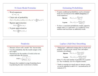
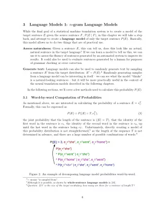
N-Gram Language Models • What? – LMs assign probabilities to sequences of tokens • Why? – Autocomplete for phones/websearch – Statistical machine translation – Speech recognition – Handwriting recognition • How? – Based on previous word histories – n-gram = consecutive sequences of tokens

Noam Chomsky Fred Jelinek But it must be recognized that the notion Anytime a linguist leaves the group “probability of a sentence” is an entirely the recognition rate goes up. (1988) useless one, under any known interpretation of this term. (1969, p. 57)

N-Gram Language Models N=1 (unigrams) This is a sentence Unigrams: This, is, a, sentence Sentence of length s , how many unigrams?

N-Gram Language Models N=2 (bigrams) This is a sentence Bigrams: This is, is a, a sentence Sentence of length s , how many bigrams?

N-Gram Language Models N=3 (trigrams) This is a sentence Trigrams: This is a, is a sentence Sentence of length s , how many trigrams?

Computing Probabilities [chain rule]

Approximating Probabilities Basic idea: limit history to fixed number of words N (Markov Assumption) N=1: Unigram Language Model

Approximating Probabilities Basic idea: limit history to fixed number of words N (Markov Assumption) N=2: Bigram Language Model

Approximating Probabilities Basic idea: limit history to fixed number of words N (Markov Assumption) N=3: Trigram Language Model

Building N-Gram Language Models • Use existing sentences to compute n-gram probability estimates (training) • Terminology: – N = total number of words in training data (tokens) – V = vocabulary size or number of unique words (types) – C( w 1 ,..., w k ) = frequency of n-gram w 1 , ..., w k in training data – P( w 1 , ..., w k ) = probability estimate for n-gram w 1 ... w k – P( w k | w 1 , ..., w k-1 ) = conditional probability of producing w k given the history w 1 , ... w k-1 What’s the vocabulary size?

Vocabulary Size: Heaps’ Law M  M is vocabulary size b kT T is collection size (number of documents) k and b are constants Typically, k is between 30 and 100, b is between 0.4 and 0.6 • Heaps’ Law: linear in log -log space • Vocabulary size grows unbounded!

Heaps’ Law for RCV1 k = 44 b = 0.49 First 1,000,020 terms: Predicted = 38,323 Actual = 38,365 Reuters-RCV1 collection: 806,791 newswire documents (Aug 20, 1996-August 19, 1997) Manning, Raghavan, Schütze, Introduction to Information Retrieval (2008)

Building N-Gram Models • Compute maximum likelihood estimates for individual n-gram probabilities – Unigram: – Bigram: • Uses relative frequencies as estimates

Example: Bigram Language Model <s> I am Sam </s> <s> Sam I am </s> I do not like green eggs and ham <s> </s> Training Corpus P( I | <s> ) = 2/3 = 0.67 P( Sam | <s> ) = 1/3 = 0.33 P( am | I ) = 2/3 = 0.67 P( do | I ) = 1/3 = 0.33 P( </s> | Sam )= 1/2 = 0.50 P( Sam | am) = 1/2 = 0.50 ... Bigram Probability Estimates Note: We don’t ever cross sentence boundaries

More Context, More Work • Larger N = more context – Lexical co-occurrences – Local syntactic relations • More context is better? • Larger N = more complex model – For example, assume a vocabulary of 100,000 – How many parameters for unigram LM? Bigram? Trigram? • Larger N has another problem…

Data Sparsity P( I | <s> ) = 2/3 = 0.67 P( Sam | <s> ) = 1/3 = 0.33 P( am | I ) = 2/3 = 0.67 P( do | I ) = 1/3 = 0.33 P( </s> | Sam )= 1/2 = 0.50 P( Sam | am) = 1/2 = 0.50 ... Bigram Probability Estimates P(I like ham) = P( I | <s> ) P( like | I ) P( ham | like ) P( </s> | ham ) = 0 Why is this bad?

Data Sparsity • Serious problem in language modeling! • Becomes more severe as N increases – What’s the tradeoff? • Solution 1: Use larger training corpora – But Zipf’s Law • Solution 2: Assign non-zero probability to unseen n-grams – Known as smoothing

Smoothing • Zeros are bad for any statistical estimator – Need better estimators because MLEs give us a lot of zeros – A distribution without zeros is “smoother” • The Robin Hood Philosophy: Take from the rich (seen n-grams) and give to the poor (unseen n- grams) – And thus also called discounting – Critical: make sure you still have a valid probability distribution!

Laplace’s Law • Simplest and oldest smoothing technique • Just add 1 to all n-gram counts including the unseen ones • So, what do the revised estimates look like?

Laplace’s Law: Probabilities Unigrams Bigrams Careful, don’t confuse the N’s!

Laplace’s Law: Frequencies Expected Frequency Estimates Relative Discount

Laplace’s Law • Bayesian estimator with uniform priors • Moves too much mass over to unseen n-grams • We can add a fraction of 1 instead – add 0 < γ < 1 to each count instead

Also: backoff Models • Consult different models in order depending on specificity (instead of all at the same time) • The most detailed model for current context first and, if that doesn’t work, back off to a lower model • Continue backing off until you reach a model that has some counts • In practice: Kneser-Ney smoothing (J&M 4.9.1)

Explicitly Modeling OOV • Fix vocabulary at some reasonable number of words • During training: – Consider any words that don’t occur in this list as unknown or out of vocabulary (OOV) words – Replace all OOVs with the special word <UNK> – Treat <UNK> as any other word and count and estimate probabilities • During testing: – Replace unknown words with <UNK> and use LM – Test set characterized by OOV rate (percentage of OOVs)

Evaluating Language Models • Information theoretic criteria used • Most common: Perplexity assigned by the trained LM to a test set • Perplexity: How surprised are you on average by what comes next ? – If the LM is good at knowing what comes next in a sentence ⇒ Low perplexity (lower is better)