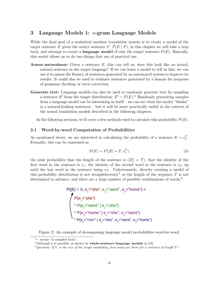
3 Language Models 1: n -gram Language Models While the final goal of - PDF document

3 Language Models 1: n -gram Language Models While the final goal of a statistical machine translation system is to create a model of the target sentence E given the source sentence F , P ( E | F ), in this chapter we will take a step back, and attempt to create a language model of only the target sentence P ( E ). Basically, this model allows us to do two things that are of practical use. Assess naturalness: Given a sentence E , this can tell us, does this look like an actual, natural sentence in the target language? If we can learn a model to tell us this, we can use it to assess the fluency of sentences generated by an automated system to improve its results. It could also be used to evaluate sentences generated by a human for purposes of grammar checking or error correction. Generate text: Language models can also be used to randomly generate text by sampling a sentence E 0 from the target distribution: E 0 ⇠ P ( E ). 4 Randomly generating samples from a language model can be interesting in itself – we can see what the model “thinks” is a natural-looking sentences – but it will be more practically useful in the context of the neural translation models described in the following chapters. In the following sections, we’ll cover a few methods used to calculate this probability P ( E ). 3.1 Word-by-word Computation of Probabilities As mentioned above, we are interested in calculating the probability of a sentence E = e T 1 . Formally, this can be expressed as P ( E ) = P ( | E | = T, e T 1 ) , (3) the joint probability that the length of the sentence is ( | E | = T ), that the identity of the first word in the sentence is e 1 , the identity of the second word in the sentence is e 2 , up until the last word in the sentence being e T . Unfortunately, directly creating a model of this probability distribution is not straightforward, 5 as the length of the sequence T is not determined in advance, and there are a large number of possible combinations of words. 6 P(|E| = 3, e 1 =”she”, e 2 =”went”, e 3 =”home”) = P(e 1 =“she”) * P(e 2 =”went” | e 1 =“she”) * P(e 3 =”home” | e 1 =“she”, e 2 =”went”) * P(e 4 =”</s>” | e 1 =“she”, e 2 =”went”, e 3 =”home”) Figure 2: An example of decomposing language model probabilities word-by-word. 4 ∼ means “is sampled from”. 5 Although it is possible, as shown by whole-sentence language models in [10]. 6 Question: If V is the size of the target vocabulary, how many are there for a sentence of length T ? 6

i am from pittsburgh . i study at a university . my mother is from utah . P(e 2 =am | e 1 =i) = c(e 1 =i, e 2 =am)/c(e 1 =i) = 1 / 2 = 0.5 P(e 2 =study | e 1 =i) = c(e 1 =i, e 2 =study)/c(e 1 =i) = 1 / 2 = 0.5 Figure 3: An example of calculating probabilities using maximum likelihood estimation. As a way to make things easier, it is common to re-write the probability of the full sen- tence as the product of single-word probabilities. This takes advantage of the fact that a joint probability – for example P ( e 1 , e 2 , e 3 ) – can be calculated by multiplying together con- ditional probabilities for each of its elements. In the example, this means that P ( e 1 , e 2 , e 3 ) = P ( e 1 ) P ( e 2 | e 1 ) P ( e 3 | e 1 , e 2 ). Figure 2 shows an example of this incremental calculation of probabilities for the sentence “she went home”. Here, in addition to the actual words in the sentence, we have introduced an implicit sentence end (“ h /s i ”) symbol, which we will indicate when we have terminated the sentence. Stepping through the equation in order, this means we first calculate the probability of “she” coming at the beginning of the sentence, then the probability of “went” coming next in a sentence starting with “she”, the probability of “home” coming after the sentence prefix “she went”, and then finally the sentence end symbol “ h /s i ” after “she went home”. More generally, we can express this as the following equation: T +1 Y P ( e t | e t � 1 P ( E ) = ) (4) 1 t =1 where e T +1 = h /s i . So coming back to the sentence end symbol h /s i , the reason why we introduce this symbol is because it allows us to know when the sentence ends. In other words, by examining the position of the h /s i symbol, we can determine the | E | = T term in our original LM joint probability in Equation 3. In this example, when we have h /s i as the 4th word in the sentence, we know we’re done and our final sentence length is 3. Once we have the formulation in Equation 4, the problem of language modeling now becomes a problem of calculating the next word given the previous words P ( e t | e t � 1 ). This 1 is much more manageable than calculating the probability for the whole sentence, as we now have a fixed set of items that we are looking to calculate probabilities for. The next couple of sections will show a few ways to do so. 3.2 Count-based n -gram Language Models The first way to calculate probabilities is simple: prepare a set of training data from which we can count word strings, count up the number of times we have seen a particular string of words, and divide it by the number of times we have seen the context. This simple method, can be expressed by the equation below, with an example shown in Figure 3 c prefix ( e t 1 ) P ML ( e t | e t � 1 ) = ) . (5) 1 c prefix ( e t � 1 1 7

Here c prefix ( · ) is the count of the number of times this particular word string appeared at the beginning of a sentence in the training data. This approach is called maximum likelihood estimation (MLE, details later in this chapter), and is both simple and guaranteed to create a model that assigns a high probability to the sentences in training data. However, let’s say we want to use this model to assign a probability to a new sentence that we’ve never seen before. For example, if we want to calculate the probability of the sentence “i am from utah .” based on the training data in the example. This sentence is extremely similar to the sentences we’ve seen before, but unfortunately because the string “i am from utah” has not been observed in our training data, c prefix (i , am , from , utah) = 0, P ( e 4 = utah | e 1 = i , e 2 = am , e 3 = from) becomes zero, and thus the probability of the whole sentence as calculated by Equation 5 also becomes zero. In fact, this language model will assign a probability of zero to every sentence that it hasn’t seen before in the training corpus, which is not very useful, as the model loses ability to tell us whether a new sentence a system generates is natural or not, or generate new outputs. To solve this problem, we take two measures. First, instead of calculating probabilities from the beginning of the sentence, we set a fixed window of previous words upon which we will base our probability calculations, approximating the true probability. If we limit our context to n � 1 previous words, this would amount to: P ( e t | e t � 1 ) ⇡ P ML ( e t | e t � 1 t � n +1 ) . (6) 1 Models that make this assumption are called n -gram models . Specifically, when models where n = 1 are called unigram models, n = 2 bigram models, n = 3 trigram models, and n � 4 four-gram, five-gram, etc. The parameters θ of n -gram models consist of probabilities of the next word given n � 1 previous words: t − n +1 = P ( e t | e t � 1 t � n +1 ) , (7) θ e t and in order to train an n -gram model, we have to learn these parameters from data. 7 In the simplest form, these parameters can be calculated using maximum likelihood estimation as follows: t � n +1 ) = c ( e t t � n +1 ) t − n +1 = P ML ( e t | e t � 1 θ e t t � n +1 ) , (8) c ( e t � 1 where c ( · ) is the count of the word string anywhere in the corpus. Sometimes these equations will reference e t � n +1 where t � n + 1 < 0. In this case, we assume that e t � n +1 = h s i where h s i is a special sentence start symbol. If we go back to our previous example and set n = 2, we can see that while the string “i am from utah .” has never appeared in the training corpus, “i am”, “am from”, “from utah”, “utah .”, and “. h /s i ” are all somewhere in the training corpus, and thus we can patch together probabilities for them and calculate a non-zero probability for the whole sentence. 8 However, we still have a problem: what if we encounter a two-word string that has never appeared in the training corpus? In this case, we’ll still get a zero probability for that particular two-word string, resulting in our full sentence probability also becoming zero. n - gram models fix this problem by smoothing probabilities, combining the maximum likelihood 7 Question: How many parameters does an n -gram model with a particular n have? 8 Question: What is this probability? 8