Neural Language Models CMSC 723 / LING 723 / INST 725 M ARINE C - PowerPoint PPT Presentation
Neural Language Models CMSC 723 / LING 723 / INST 725 M ARINE C ARPUAT marine@cs.umd.edu With slides from Graham Neubig and Philipp Koehn Roadmap Modeling Sequences First example: language model What are n-gram models? How to
Neural Language Models CMSC 723 / LING 723 / INST 725 M ARINE C ARPUAT marine@cs.umd.edu With slides from Graham Neubig and Philipp Koehn
Roadmap • Modeling Sequences – First example: language model – What are n-gram models? – How to estimate them? – How to evaluate them? – Neural language models
Probabilistic Language Modeling • Goal: compute the probability of a sentence or sequence of words P(W) = P(w 1 ,w 2 ,w 3 ,w 4 ,w 5 … w n ) • Related task: probability of an upcoming word P(w 5 |w 1 ,w 2 ,w 3 ,w 4 ) • A model that computes either of these: P(W) or P(w n |w 1 ,w 2 …w n-1 ) is called a language model .
Evaluation: How good is our model? • Does our language model prefer good sentences to bad ones? – Assign higher probability to “real” or “frequently observed” sentences • Than “ungrammatical” or “rarely observed” sentences? • Extrinsic vs intrinsic evaluation
Intrinsic evaluation: intuition • The Shannon Game: – How well can we predict the next word? mushrooms 0.1 pepperoni 0.1 anchovies 0.01 I always order pizza with cheese and ____ …. The 33 rd President of the US was ____ fried rice 0.0001 I saw a ____ …. and 1e-100 – Unigrams are terrible at this game. (Why?) • A better model of a text assigns a higher probability to the word that actually occurs
Intrinsic evaluation metric: perplexity The best language model is one that best predicts an unseen test set • Gives the highest P(sentence) - 1 = PP ( W ) P ( w 1 w 2 ... w N ) N Perplexity is the inverse probability of the test set, normalized by the number of 1 words: = N P ( w 1 w 2 ... w N ) Chain rule: For bigrams: Minimizing perplexity is the same as maximizing probability
Perplexity as branching factor • Let’s suppose a sentence consisting of N random digits • What is the perplexity of this sentence according to a model that assign P=1/10 to each digit?
Lower perplexity = better model • Training 38 million words, test 1.5 million words, WSJ N-gram Unigram Bigram Trigram Order Perplexity 962 170 109
Pros and cons of n-gram models • N-gram models – Really easy to build, can train on billions and billions of words – Smoothing helps generalize to new data – Only work well for word prediction if the test corpus looks like the training corpus – Only capture short distance context “Smarter” LMs can address some of these issues, but they are order of magnitudes slower…
Roadmap • Modeling Sequences – First example: language model – What are n-gram models? – How to estimate them? – How to evaluate them? – Neural language models
Aside NE NEURAL AL NE NETWO WORKS KS
Recall the person/not-person classification problem Given an introductory sentence in Wikipedia predict whether the article is about a person
Formalizing binary prediction
The Perceptron: a “machine” to calculate a weighted sum φ “A” = 1 0 φ “site” = 1 -3 φ “located” = 1 0 φ “Maizuru” = 1 0 𝐽 -1 0 sign 𝑥 𝑗 ⋅ ϕ 𝑗 𝑦 φ “,” = 2 𝑗=1 0 φ “in” = 1 0 φ “Kyoto” = 1 2 0 φ “priest” = 0 φ “black” = 0
The Perceptron: Geometric interpretation O X O X O X
The Perceptron: Geometric interpretation O X O X O X
Limitation of perceptron ● can only find linear separations between positive and negative examples X O O X
Neural Networks ● Connect together multiple perceptrons φ “A” = 1 φ “site” = 1 φ “located” = 1 φ “Maizuru” = 1 -1 φ “,” = 2 φ “in” = 1 φ “Kyoto” = 1 φ “priest” = 0 φ “black” = 0 ● Motivation: Can represent non-linear functions!
Neural Networks: key terms • Input (aka features) • Output • Nodes • Layers φ “A” = 1 • Activation function φ “site” = 1 (non-linear) φ “located” = 1 φ “Maizuru” = 1 -1 φ “,” = 2 φ “in” = 1 φ “Kyoto” = 1 • Multi-layer φ “priest” = 0 perceptron φ “black” = 0
Example ● Create two classifiers w 0,0 φ 0 [0] 1 φ 0 (x 1 ) = {-1, 1} φ 0 (x 2 ) = {1, 1} 1 φ 0 [1] φ 1 [0] sign φ 0 [1] X O -1 1 b 0,0 φ 0 [0] w 0,1 O X φ 0 [0] -1 φ 0 (x 3 ) = {-1, -1} φ 0 (x 4 ) = {1, -1} -1 φ 0 [1] φ 1 [1] sign -1 1 b 0,1
Example ● These classifiers map to a new space φ 1 (x 3 ) = {-1, 1} φ 0 (x 1 ) = {-1, 1} φ 0 (x 2 ) = {1, 1} φ 1 [1] φ 2 O X O φ 1 φ 1 [0] X O X O φ 1 (x 1 ) = {-1, -1} φ 1 (x 2 ) = {1, -1} φ 0 (x 3 ) = {-1, -1} φ 0 (x 4 ) = {1, -1} φ 1 (x 4 ) = {-1, -1} 1 φ 1 [0] 1 -1 -1 φ 1 [1] -1 -1
Example ● In new space, the examples are linearly separable! φ 0 (x 1 ) = {-1, 1} φ 0 (x 2 ) = {1, 1} φ 0 [1] X O φ 0 [0] 1 φ 2 [0] = y 1 1 O X φ 0 (x 3 ) = {-1, -1} φ 0 (x 4 ) = {1, -1} φ 1 [1] 1 φ 1 (x 3 ) = {-1, 1} O φ 1 [0] 1 -1 φ 1 [0] -1 φ 1 (x 1 ) = {-1, -1} X φ 1 [1] -1 O φ 1 (x 2 ) = {1, -1} -1 φ 1 (x 4 ) = {-1, -1}
Example wrap-up: Forward propagation ● The final net φ 0 [0] 1 1 φ 0 [1] φ 1 [0] tanh 1 -1 1 φ 0 [0] φ 2 [0] -1 tanh 1 -1 φ 0 [1] φ 1 [1] tanh -1 1 1 1
Softmax Function for multiclass classification ● Sigmoid function for multiple classes 𝑓 𝐱⋅ϕ 𝑦,𝑧 Current class 𝑄 𝑧 ∣ 𝑦 = 𝑧 𝑓 𝐱⋅ϕ 𝑦, 𝑧 Sum of other classes ● Can be expressed using matrix/vector ops 𝐬 = exp 𝐗 ⋅ ϕ 𝑦 𝐪 = 𝐬 𝑠 𝑠∈𝐬 24
Stochastic Gradient Descent Online training algorithm for probabilistic models w = 0 for I iterations for each labeled pair x, y in the data w += α * dP(y|x)/dw In other words For every training example, calculate the gradient • (the direction that will increase the probability of y) Move in that direction, multiplied by learning rate α •
Gradient of the Sigmoid Function Take the derivative of the probability 0.4 dp(y|x)/dw*phi(x) 𝑓 𝐱⋅ϕ 𝑦 𝑒 𝑒 0.3 𝑒𝑥 𝑄 𝑧 = 1 ∣ 𝑦 = 1 + 𝑓 𝐱⋅ϕ 𝑦 𝑒𝑥 0.2 𝑓 𝐱⋅ϕ 𝑦 0.1 = ϕ 𝑦 1 + 𝑓 𝐱⋅ϕ 𝑦 2 0 -10 0 10 w*phi(x) 𝑓 𝐱⋅ϕ 𝑦 𝑒 𝑒 𝑒𝑥 𝑄 𝑧 = −1 ∣ 𝑦 = 1 − 1 + 𝑓 𝐱⋅ϕ 𝑦 𝑒𝑥 𝑓 𝐱⋅ϕ 𝑦 = −ϕ 𝑦 1 + 𝑓 𝐱⋅ϕ 𝑦 2
Learning: We Don't Know the Derivative for Hidden Units! For NNs, only know correct tag for last layer 𝐢 𝑦 w 1 𝑒𝑄 𝑧 = 1 ∣ 𝐲 = ? 𝑒𝐱 𝟐 𝑓 𝐱 𝟓 ⋅𝐢 𝑦 𝑒𝑄 𝑧 = 1 ∣ 𝐲 = 𝐢 𝑦 1 + 𝑓 𝐱 𝟓 ⋅𝐢 𝑦 2 𝑒𝐱 𝟓 w 2 w 4 ϕ 𝑦 y=1 𝑒𝑄 𝑧 = 1 ∣ 𝐲 = ? w 3 𝑒𝐱 𝟑 𝑒𝑄 𝑧 = 1 ∣ 𝐲 = ? 𝑒𝐱 𝟒
Answer: Back-Propagation Calculate derivative with chain rule 𝑒𝑄 𝑧 = 1 ∣ 𝑦 = 𝑒𝑄 𝑧 = 1 ∣ 𝑦 𝑒𝐱 𝟓 𝐢 𝐲 𝑒ℎ 1 𝐲 𝑒𝐱 𝟐 𝑒𝐱 𝟓 𝐢 𝐲 𝑒ℎ 1 𝐲 𝑒𝐱 𝟐 𝑓 𝐱 𝟓 ⋅𝐢 𝑦 𝑥 1,4 1 + 𝑓 𝐱 𝟓 ⋅𝐢 𝑦 2 Error of Weight Gradient of next unit (δ 4 ) this unit 𝑒𝑄 𝑧 = 1 ∣ 𝐲 = 𝑒ℎ 𝑗 𝐲 In General δ 𝑘 𝑥 𝑗,𝑘 𝐱 𝐣 𝑒𝐱 𝐣 Calculate i based 𝑘 on next units j :
Backpropagation = Gradient descent + Chain rule
Feed Forward Neural Nets All connections point forward ϕ 𝑦 y It is a directed acyclic graph (DAG)
Neural Networks • Non-linear classification • Prediction: forward propagation – Vector/matrix operations + non-linearities • Training: backpropagation + stochastic gradient descent For more details, see Cho chap 3 or CIML Chap 7
Aside NE NEURAL AL NE NETWO WORKS KS
Back to language modeling…
Representing words • “one hot vector” dog = [ 0, 0, 0, 0, 1, 0, 0, 0 …] cat = [ 0, 0, 0, 0, 0, 0, 1, 0 …] eat = [ 0, 1, 0, 0, 0, 0, 1, 0 …] • That’s a large vector! practical solutions: – limit to most frequent words (e.g., top 20000) – cluster words into classes • WordNet classes, frequency binning, etc.
Feed-Forward Neural Language Model Map each word into a lower-dimensional real-valued space using shared weight matrix C Embedding layer Bengio et al. 2003
Word Embeddings • Neural language models produce word embeddings as a by product • Words that occurs in similar contexts tend to have similar embeddings • Embeddings are useful features in many NLP tasks [Turian et al. 2009]
Word embeddings illustrated
Recurrent Neural Networks
Recurrent Neural Nets (RNN) Part of the node outputs return as input 𝐢 𝐮−𝟐 ϕ 𝐮 𝑦 y Why? It is possible to “memorize”
Training: backpropagation through time After processing a few training examples, Update through the unfolded recurrent neural network
Recurrent neural language models • Hidden layer plays double duty – Memory of the network – Continuous space representation to predict output words • Other more elaborate architectures – Long Short Term Memory – Gated Recurrent Units
Recommend
More recommend
Explore More Topics
Stay informed with curated content and fresh updates.
