CS533 No experiment is ever a complete failure. It can always serve - PDF document

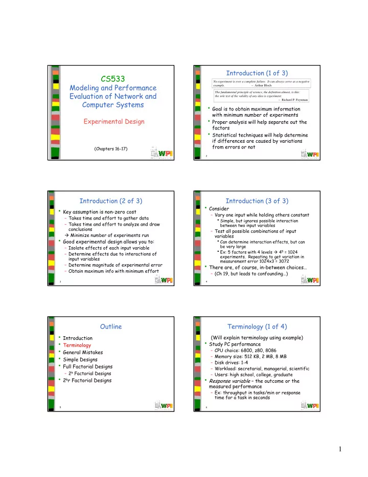
Introduction (1 of 3) CS533 No experiment is ever a complete failure. It can always serve as a negative Modeling and Performance example. – Arthur Bloch Evaluation of Network and The fundamental principle of science, the definition almost, is this: the sole test of the validity of any idea is experiment. – Richard P. Feynman Computer Systems • Goal is to obtain maximum information with minimum number of experiments • Proper analysis will help separate out the Experimental Design factors • Statistical techniques will help determine if differences are caused by variations from errors or not (Chapters 16-17) 1 2 Introduction (2 of 3) Introduction (3 of 3) • Consider • Key assumption is non-zero cost – Vary one input while holding others constant – Takes time and effort to gather data • Simple, but ignores possible interaction – Takes time and effort to analyze and draw between two input variables conclusions – Test all possible combinations of input � Minimize number of experiments run variables • Good experimental design allows you to: • Can determine interaction effects, but can be very large – Isolate effects of each input variable • Ex: 5 factors with 4 levels � 4 5 = 1024 – Determine effects due to interactions of experiments. Repeating to get variation in input variables measurement error 1024x3 = 3072 • There are, of course, in-between choices… – Determine magnitude of experimental error – Obtain maximum info with minimum effort – (Ch 19, but leads to confounding…) 3 4 Outline Terminology (1 of 4) • Introduction (Will explain terminology using example) • Study PC performance • Terminology • General Mistakes – CPU choice: 6800, z80, 8086 • Simple Designs – Memory size: 512 KB, 2 MB, 8 MB – Disk drives: 1-4 • Full Factorial Designs – Workload: secretarial, managerial, scientific – 2 k Factorial Designs – Users: high school, college, graduate • 2 k r Factorial Designs • Response variable – the outcome or the measured performance – Ex: throughput in tasks/min or response time for a task in seconds 5 6 1

Terminology (2 of 4) Terminology (3 of 4) • Factors – each variable that affects • Secondary factors – of less importance response – Ex: maybe user type not as important • Replication – repetition of all or some – Ex: CPU, memory, disks, workload, user – Also called predictor variables or predictors experiments • Levels – the different values factors can – Ex: if run three times, then three take replications • Design – specification of the replication, – EX: CPU 3, memory 3, disks 4, workload 3, users 3 factors, levels – Also called treatment – Ex: Specify all factors, at above levels with • Primary factors – those of most important 5 replications so 3x3x4x3x3 = 324 time 5 replications yields 1215 total interest – Ex: maybe CPU and memory the most 7 8 Terminology (4 of 4) Outline • Interaction – two factors A and B interact if one • Introduction • Terminology shows dependence upon another – Ex: non-interacting factor since A always increases • General Mistakes by 2 A 1 • Simple Designs A 1 A 2 A 2 • Full Factorial Designs B 1 3 5 B 2 6 8 – 2 k Factorial Designs B 1 B 2 • 2 k r Factorial Designs – Ex: interacting factors since A change depends upon B A 1 A 1 A 2 B 1 3 5 A 2 B 2 6 9 9 10 B 1 B 2 Common Mistakes in Experiments Common Mistakes in Experiments (1 of 2) (2 of 2) • Interactions are ignored. • Variation due to experimental error is ignored. – Often effect of one factor depend upon another. – Measured values have randomness due to Ex: effects of cache may depend upon size of measurement error. Do not assign (or assume) all program. Need to move beyond one-factor-at-a- variation is due to factors. time designs • Important parameters not controlled. • Too many experiments are conducted. – All parameters (factors) should be listed and – Rather than running all factors, all levels, at all accounted for, even if not all are varied. combinations, break into steps • Effects of different factors not isolated. – First step, few factors and few levels – May vary several factors simultaneously and then • Determine which factors are significant not be able to attribute change to any one. • Two levels per factor (details later) – Use of simple designs (next topic) may help but have – More levels added at later design, as appropriate their own problems. 11 12 2

Outline Simple Designs • Introduction • Start with typical configuration • Vary one factor at a time • Terminology • Ex: typical may be PC with z80, 2 MB RAM, 2 • General Mistakes disks, managerial workload by college student • Simple Designs – Vary CPU, keeping everything else constant, and compare • Full Factorial Designs – Vary disk drives, keeping everything else constant, – 2 k Factorial Designs and compare • Given k factors, with i th having n i levels • 2 k r Factorial Designs Total = 1 + Σ ( n i -1) for i = 1 to k • Example: in workstation study 1 + (3-1) + (3-1) + (4-1) + (3-1) + (3-1) + (3-1) = 14 • But may ignore interaction (Example next) 13 14 Example of Interaction of Factors Outline • Consider response time vs. memory size • Introduction • Terminology and degree of multiprogramming • General Mistakes Degree 32 MB 64 MB 128MB • Simple Designs 1 0.25 0.21 0.15 • Full Factorial Designs 2 0.52 0.45 0.36 3 0.81 0.66 0.50 – 2 k Factorial Designs 4 1.50 1.45 0.70 • 2 k r Factorial Designs • If fixed degree 3, mem 64 and vary one at a time, may miss interaction – Example: degree 4, non-linear response time with memory 15 16 2 k Factorial Designs Full Factorial Designs • Every possible combination at all levels of all Twenty percent of the jobs account for 80% of the resource consumption. – Pareto’s Law factors • Given k factors, with i th having n i levels • Very often, many levels at each factor Total = Π n i for i = 1 to k – Ex: effect of network latency on user response time • Example: in CPU design study � there are lots of latency values to test • Often, performance continuously increases or (3 CPUs)(3 mem) (4 disks) (3 loads) (3 users) decreases over levels = 324 experiments • Advantage is can find every interaction component – Ex: response time always gets higher • Disadvantage is costs (time and money), especially – Can determine direction with min and max • For each factor, choose 2 alternatives at each since may need multiple iterations (later) • Can reduce costs by: reduce levels, reduce factors, level – 2 k factorial designs run fraction of full factorial • Then, can determine which of the factors impacts (Next, reduce levels) performance the most and study those further 17 18 3

2 2 Factorial Design (1 of 4) 2 2 Factorial Design (2 of 4) • Special case with only 2 factors • Substituting: – Easily analyzed with regression 15 = q 0 - q a - q b + q ab • Example: MIPS for Mem (4 or 16 Mbytes) and Cache 45 = q 0 + q a - q b - q ab (4 equations in (1 or 2 Kbytes) 25 = q 0 - q a + q b - q ab 4 unknowns) Mem 4MB Mem 16MB 75 = q 0 + q a + q b + q ab • Can solve to get: Cache 1 KB 15 45 Cache 2 KB 25 75 y = 40 + 20x a + 10x b + 5x a x b • Define x a = -1 if 4 Mbytes mem, +1 if 16 Mbytes • Interpret: • Define x b = -1 if 1 Kbyte cache, +1 if 2 Kbytes – Mean performance is 40 MIPS, memory effect is 20 • Performance: MIPS, cache effect is 10 MIPS and interaction effect is 5 MIPS y = q 0 + q a x a + q b x b + q ab x a x b (Generalize to easier method next) 19 20 2 2 Factorial Design (3 of 4) 2 2 Factorial Design (4 of 4) • Solving, we get: • Multiply column Exp a b y i a b ab y 1 -1 -1 y 1 1 -1 -1 1 15 entries by y i and sum q 0 = ¼( y 1 + y 2 + y 3 + y 4 ) • Dived each by 4 to 2 1 -1 y 2 1 1 -1 -1 45 q a = ¼(-y 1 + y 2 - y 3 + y 4 ) 3 -1 1 y 3 1 -1 1 -1 25 give weight in q b = ¼(-y 1 - y 2 + y 3 + y 4 ) regression model 4 1 1 y 4 1 1 1 1 75 q ab = ¼( y 1 - y 2 - y 3 + y 4 ) • Final: • Notice for q a can y = q 0 + q a x a + q b x b + 160 80 40 20 Total q ab x a x b 40 20 10 5 Ttl/4 obtain by multiplying y = 40 + 20x a + 10x b + • So: • Column “i” has all 1s 5x a x b “a” column by “y” • Columns “a” and “b” have y 1 = q 0 - q a - q b + q ab column and adding y 2 = q 0 + q a - q b - q ab all combinations of 1, -1 – Same is true for q b • Column “ab” is product of y 3 = q 0 - q a + q b - q ab and q ab y 4 = q 0 + q a + q b + q ab column “a” and “b” 21 22 Allocation of Variation (1 of 3) Allocation of Variation (2 of 3) • Importance of a factor measured by • For a 2 2 design, variation is in 3 parts: proportion of total variation in response – SST = 2 2 q 2 a + 2 2 q 2 b + 2 2 q 2 (Derivation 17.1, p.287) • Portion of total variation: ab explained by the factor – Thus, if two factors explain 90% and 5% of – of a is 2 2 q 2 the response, then the second may be a – of b is 2 2 q 2 ignored b • Ex: capacity factor (768 Kbps or 10 Mbps) – of ab is 2 2 q 2 • Thus, SST = SSA + SSB + SSAB ab versus TCP version factor (Reno or Sack) • Sample variance of y • And fraction of variation explained by a: 2 = Σ (y i – y) 2 / (2 2 – 1) s y = SSA/SST • With numerator being total variation, or – Note, may not explain the same fraction of Sum of Squares Total (SST) variance since that depends upon errors+ SST = Σ (y i – y) 2 23 24 4