= x ... What is a Statistic ? What are Statistic s ? A - PDF document
Why do we need statistics? CS533 Modeling and Performance 1. Noise, noise, noise, noise, noise! Evaluation of Network and Computer Systems Statistics for Performance Evaluation OK not really this type of noise (Chapters 12-15) Why Do
Why do we need statistics? CS533 Modeling and Performance 1. Noise, noise, noise, noise, noise! Evaluation of Network and Computer Systems Statistics for Performance Evaluation OK – not really this type of noise (Chapters 12-15) Why Do We Need Statistics? Why Do We Need Statistics? “Impossible things usually don’t happen.” 2. Aggregate data into meaningful - Sam Treiman, Princeton University • Statistics helps us quantify “usually.” information. 445 446 397 226 388 3445 188 1002 47762 432 54 12 98 345 2245 8839 77492 472 565 999 1 34 882 545 4022 827 572 597 364 = x ... What is a Statistic ? What are Statistic s ? • • “A quantity that is computed from a “Lies, damn lies, and statistics!” • sample [of data].” “A collection of quantitative data.” • Merriam-Webster “A branch of mathematics dealing with → A single number used to summarize a the collection, analysis, interpretation, larger collection of values. and presentation of masses of numerical data.” Merriam-Webster → We are most interested in analysis and interpretation here. 1
Objectives Outline • • Introduction Provide intuitive conceptual background • Basics for some standard statistical tools. • Indices of Central Tendency – Draw meaningful conclusions in presence of noisy measurements. • Indices of Dispersion – Allow you to correctly and intelligently • Comparing Systems apply techniques in new situations. • Misc → Don’t simply plug and crank from a • Regression formula! • ANOVA Basics (1 of 3) Basics (2 of 3) • Independent Events: • Coefficient of Variation: – One event does not affect the other – Ratio of standard deviation to mean – Knowing probability of one event does not change – C.O.V. = σ / µ estimate of another • Cumulative Distribution (or Density) Function: • Covariance: – F x (a) = P(x<=a) – Degree two random variables vary with each • Mean (or Expected Value): other – Mean µ = E(x) = Σ (p i x i ) for i over n – Cov = σ 2 xy = E[(x- µ x )(y- µ y )] • Variance: – Two independent variables have Cov of 0 – Square of the distance between x and the mean • Correlation: • (x- µ) 2 – Var(x) = E[(x- µ) 2 ] = Σ p i (x i - µ) 2 – Normalized Cov (between –1 and 1) – Variance is often σ . Square root of variance, σ 2 , is – ρ xy = σ 2 xy / σ x σ y standard deviation – Represents degree of linear relationship Basics (3 of 3) Outline • Quantile: • Introduction • Basics – The x value of the CDF at α • Indices of Central Tendency – Denoted x α , so F(x α ) = α – Often want .25, .50, .75 • Indices of Dispersion • Median: • Comparing Systems – The 50-percentile (or, .5-quantile) • Misc • Mode: • Regression – The most likely value of x i • Normal Distribution • ANOVA – Most common distribution used, “bell” curve 2
Summarizing Data by a Single Relationship Between Mean, Number Median, Mode • Indices of central tendency mean modes median • Three popular: mean, median, mode mode mean • Mean – sum all observations, divide by num pdf pdf median f(x) f(x) • Median – sort in increasing order, take no mode middle pdf • Mode – plot histogram and take largest mean (a) (b) f(x) median bucket mode mode • Mean can be affected by outliers, while median (c) median pdf pdf median or mode ignore lots of info f(x) mean f(x) • Mean has additive properties (mean of a mean sum is the sum of the means), but not (d) median or mode (d) Guidelines in Selecting Index of Examples for Index of Central Central Tendency Tendency Selection • Is it categorical? • Most used resource in a system? – � yes, use mode – Categorical, so use mode • Ex: most frequent microprocessor • Response time? • Is total of interest? – Total is of interest, so use mean – � yes, use mean • Load on a computer? • Ex: total CPU time for query (yes) – Probably highly skewed, so use median • Ex: number of windows on screen in query (no) • Average configuration of number of disks, • Is distribution skewed? amount of memory, speed of network? – � yes, use median – Probably skewed, so use median – � no, use mean Common Misuses of Means (1 of 2) Common Misuses of Means (2 of 2) • Using mean of significantly different values • Multiplying means – Just because mean is right, does not say it is – Mean of product equals product of means if useful two variables are independent. But: • Ex: two samples of response time, 10 ms and • if x,y are correlated E(xy) != E(x)E(y) 1000 ms. Mean is 505 ms but useless. – Ex: mean users system 23, mean processes • Using mean without regard to skew per user is 2. What is the mean system processes? Not 46! – Does not well-represent data if skewed • Ex: sys A: 10, 9, 11, 10, 10 (mean 10, mode 10) � Processes determined by load, so when load • Ex: sys B: 5, 5, 5, 4, 31 (mean 10, mode 5) high then users have fewer. Instead, must measure total processes and average. • Mean of ratio with different bases (later) 3
Geometric Mean (1 of 2) Geometric Mean (2 of 2) • Previous mean was arithmetic mean • Other examples of metrics that work in a – Used when sum of samples is of interest multiplicative manner: – Geometric mean when product is of interest • Multiply n values {x 1 , x 2 , …, x n } and take n th root: – Cache hit ratios over several levels • And cache miss ratios x = ( Π x i ) 1/ n • Example: measure time of network layer – Percentage of performance improvement improvement, where 2x layer 1 and 2x layer 2 between successive versions equals 4x improvement. – Average error rate per hop on a multi-hop • Layer 7 improves 18%, 6 13%, 5, 11%, 4 8%, 3 10%, path in a network 2 28%, 1 5% • So, geometric mean per layer: – [(1.18)(1.13)(1.11)(1.08)(1.10)(1.28)(1.05)] 1/7 – 1 – Average improvement per layer is 0.13, or 13% Harmonic Mean (1 of 2) Harmonic Mean (2 of 2) • Ex: if different benchmarks (m i ), then sum • Harmonic mean of samples {x 1 , x 2 , …, x n } is: of m i /t i does not make sense n / (1/x 1 + 1/x 2 + … + 1/x n ) • Instead, use weighted harmonic mean • Use when arithmetic mean works for 1/x • Ex: measurement of elapsed processor n / (w 1 /x 1 + w 2 /x 2 + … + w 3 /x n ) – where w 1 + w 2 + .. + w n = 1 benchmark of m instructions. The i th • In example, perhaps choose weights takes t i seconds. MIPS x i is m /t i proportional to size of benchmarks – Since sum of instructions matters, can use – w i = m i / (m 1 + m 2 + .. + m n ) harmonic mean • So, weighted harmonic mean = n / [1/( m /t 1 ) + 1/( m /t 2 ) + … + 1/( m /t n )] (m 1 + m 2 + .. + m n ) / (t 1 + t 2 + .. + t n ) = m / [(1/ n )(t 1 + t 2 + … + t n ) – Reasonable, since top is total size and bottom is total time Mean of a Ratio (1 of 2) Mean of a Ratio (2 of 2) • Set of n ratios, how to summarize? • CPU utilization: • Here, if sum of numerators and sum of – For duration 1 busy 45%, 1 %45, 1 45%, 1 denominators both have meaning, the 45%, 100 20% average ratio is the ratio of averages – Sum 200%, mean != 200/5 or 40% • The base denominators (duration) are not Average(a 1 /b 1 , a 2 /b 2 , …, a n /b n ) comparable = (a 1 + a 2 + … + a n ) / (b 1 + b 2 + … + b n ) – mean = sum of CPU busy / sum of durations = [( Σ a i )/ n ] / [( Σ b i )/ n ] • Commonly used in computing mean resource = (.45+.45+.45+.45+20) / (1+1+1+1+100) = 21% utilization (example next) 4
Outline Summarizing Variability (1 of 2) • Introduction “Then there is the man who drowned crossing a stream with an average depth of six inches.” – W.I.E. Gates • Basics • Indices of Central Tendency • Summarizing by a single number is rarely • Indices of Dispersion enough � need statement about variability • Comparing Systems – If two systems have same mean, tend to prefer one with less variability • Misc • Regression • ANOVA Frequency Frequency mean mean Response Time Response Time Summarizing Variability (2 of 2) Range • Easy to keep track of • Indices of Dispersion • Record max and min, subtract – Range – min and max values observed • Mostly, not very useful: – Variance or standard deviation – Minimum may be zero – 10- and 90- percentiles – Maximum can be from outlier – ( Semi-)interquartile range • System event not related to phenomena – Mean absolute deviation studied – Maximum gets larger with more samples, so no “stable” point (Talk about each next) • However, if system is bounded, for large sample, range may give bounds Sample Variance Standard Deviation • So, use standard deviation • Sample variance (can drop word “sample” if meansing is clear) – s = sqrt(s 2 ) – s 2 = [1/( n -1)] Σ (x i – x) 2 – Same unit as mean , so can compare to mean • Ex: response times of .5, .4, .6 seconds • Notice ( n -1) since only n -1 are independent – stddev .1 seconds or 100 msecs – Also called degrees of freedom • Main problem is in units squared so – Can compare each to mean • Ratio of standard deviation to mean ? changing the units changes the answer – Called the Coefficient of Variation (C.O.V.) squared – Takes units out and shows magnitude – Ex: response times of .5, .4, .6 seconds – Ex: above is 1/5 th (or .2) for either unit Variance = 0.01 seconds squared or 10000 msecs squared 5
Recommend
More recommend
Explore More Topics
Stay informed with curated content and fresh updates.
![Sampling Sampling In [1]: % matplotlib inline from matplotlib import pyplot as plt import mxnet](https://c.sambuz.com/967442/sampling-sampling-s.webp)


