Introduction Variability in Data Summarizing variability in a data - PDF document

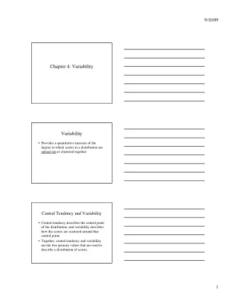
Introduction Variability in Data • Summarizing variability in a data set CS 239 • Estimating variability in sample data Experimental Methodologies for System Software Peter Reiher April 10, 2007 Lecture 3 Lecture 3 Page 1 Page 2 CS 239, Spring 2007 CS 239, Spring 2007 Summarizing Variability Why Is Variability Important? • Consider two Web servers - • A single number rarely tells the entire • Server A services all requests in 1 second story of a data set • Server B services 90% of all requests in .5 • Usually, you need to know how much seconds the rest of the data set varies from that • But 10% in 55 seconds index of central tendency • Both have mean service times of 1 second • But which would you prefer to use? Lecture 3 Lecture 3 Page 3 Page 4 CS 239, Spring 2007 CS 239, Spring 2007 Indices of Dispersion Range • Minimum and maximum values in data set • Measures of how much a data set • Can be kept track of as data values arrive varies • Variability characterized by difference –Range between minimum and maximum –Variance and standard deviation • Often not useful, due to outliers –Percentiles • Minimum tends to go to zero –Semi-interquartile range • Maximum tends to increase over time –Mean absolute deviation • Not useful for unbounded variables Lecture 3 Lecture 3 Page 5 Page 6 CS 239, Spring 2007 CS 239, Spring 2007 1

Example of Range Variance (and Its Cousins) • Sample variance is • For data set: 1 n ? ? 2 2 ? ? ? s x x 2, 5.4, -17, 2056, 445, -4.8, 84.3, 92, ? i n 1 ? i 1 27, -10 • Variance is expressed in units of the • Maximum is 2056 measured quantity squared • Minimum is -17 – Which isn’t always easy to understand • Range is 2073 • Standard deviation and the coefficient of variation are derived from variance • While arithmetic mean is 268 Lecture 3 Lecture 3 Page 7 Page 8 CS 239, Spring 2007 CS 239, Spring 2007 Variance Example Standard Deviation • For data set • The square root of the variance 2, 5.4, -17, 2056, 445, -4.8, 84.3, 92, • In the same units as the units of the 27, -10 metric • Variance is 413746.6 • So easier to compare to the metric • Given a mean of 268, what does that variance indicate? Lecture 3 Lecture 3 Page 9 Page 10 CS 239, Spring 2007 CS 239, Spring 2007 Standard Deviation Example Coefficient of Variation • For data set • The ratio of the mean and standard 2, 5.4, -17, 2056, 445, -4.8, 84.3, 92, deviation 27, -10 • Normalizes the units of these quantities • Standard deviation is 643 into a ratio or percentage • Given a mean of 268, clearly the • Often abbreviated C.O.V. standard deviation shows a lot of variability from the mean Lecture 3 Lecture 3 Page 11 Page 12 CS 239, Spring 2007 CS 239, Spring 2007 2

Coefficient of Variation Example Percentiles • Specification of how observations fall • For data set into buckets 2, 5.4, -17, 2056, 445, -4.8, 84.3, 92, • E.g., the 5-percentile is the observation 27, -10 that is at the lower 5% of the set • Standard deviation is 643 • The 95-percentile is the observation at • The mean of 268 the 95% boundary of the set • So the C.O.V. is 643/268 = 2.4 • Useful even for unbounded variables Lecture 3 Lecture 3 Page 13 Page 14 CS 239, Spring 2007 CS 239, Spring 2007 Relatives of Percentiles Calculating Quantiles • Quantiles - fraction between 0 and 1 • The ? -quantile is estimated by sorting – Instead of percentage the set – Also called fractiles • Then take the [(n-1) ? +1] th element • Deciles - percentiles at the 10% boundaries – First is 10-percentile, second is 20- –Rounding to the nearest integer percentile, etc. index • Quartiles -divide data set into four parts – 25% of sample below first quartile, etc. – Second quartile is also the median Lecture 3 Lecture 3 Page 15 Page 16 CS 239, Spring 2007 CS 239, Spring 2007 Quartile Example Interquartile Range • Yet another measure of dispersion • For data set 2, 5.4, -17, 2056, 445, -4.8, 84.3, 92, 27, • The difference between Q3 and Q1 -10 • Semi-interquartile range - – (10 observations) • Sort it: ? Q Q ? 3 1 SIQR -17, -10, -4.8, 2, 5.4, 27, 84.3, 92, 445, 2056 2 • The first quartile Q 1 is -4.8 • The third quartile Q 3 is 92 • Often interesting measure of what’s going on in the middle of the range Lecture 3 Lecture 3 Page 17 Page 18 CS 239, Spring 2007 CS 239, Spring 2007 3

Semi-Interquartile Range Mean Absolute Deviation Example • For data set • Another measure of variability -17, -10, -4.8, 2, 5.4, 27, 84.3, 92, 445, 2056 1 n ? ? • Mean absolute deviation = x x i • Q 3 is 92 n ? 1 i • Q 1 is -4.8 ? ? ? • Doesn’t require multiplication or Q Q 92 4 8 . ? ? ? 3 1 SIQR 48 square roots 2 2 • So outliers cause much of variability Lecture 3 Lecture 3 Page 19 Page 20 CS 239, Spring 2007 CS 239, Spring 2007 Mean Absolute Deviation Sensitivity To Outliers Example • For data set • From most to least, -17, -10, -4.8, 2, 5.4, 27, 84.3, 92, 445, –Range 2056 –Variance 10 x –Mean absolute deviation 1 ? ? • Mean absolute deviation = x i 10 ? –Semi-interquartile range i 1 • Or 393 Lecture 3 Lecture 3 Page 21 Page 22 CS 239, Spring 2007 CS 239, Spring 2007 So, Which Index of Dispersion Determining Distributions for Should I Use? Datasets • If a data set has a common distribution, Yes Range Bounded? that’s the best way to summarize it No • Saying a data set is uniformly Unimodal distributed is more informative than Yes C.O.V symmetrical? just giving its mean and standard No deviation Percentiles or SIQR • But always remember what you’re looking for Lecture 3 Lecture 3 Page 23 Page 24 CS 239, Spring 2007 CS 239, Spring 2007 4

Some Commonly Used Distributions Uniform Distribution • Uniform distribution • All values in a given range are equally likely • Often normalized to a range from zero to one • Normal distribution • Suggests randomness in phenomenon being tested • Exponential distribution 1 ? – Pdf: f ( x ) ? B A • There are many others ? f ( x ) x – CDF: ? x ? • Assuming 0 1 Lecture 3 Lecture 3 Page 25 Page 26 CS 239, Spring 2007 CS 239, Spring 2007 CDF for Uniform Distribution Normal Distribution • Some value of random variable is most likely – Declining probabilities of values as one moves away from this value – Equally on either side of most probable value • Extremely widely used • Generally sort of a “default distribution” – Which isn’t always right . . . Lecture 3 Lecture 3 Page 27 Page 28 CS 239, Spring 2007 CS 239, Spring 2007 PDF and CDF for Normal PDF for Normal Distribution Distribution • PDF expressed in terms of – Location parameter µ (the popular value) – Scale parameter s (how much spread) – PDF is ? ? ? 2 ? 2 ( x ) /( 2 ) e ? f ( x ) ? ? 2 – CDF doesn’t exist in closed form Lecture 3 Lecture 3 Page 29 Page 30 CS 239, Spring 2007 CS 239, Spring 2007 5

Exponential Distribution PDF of Exponential Distribution • Describes value that declines over time – E.g., failure probabilities – Described in terms of location parameter µ – And scale parameter ß – Standard exponential when µ = 0 and ß =1 • PDF: 1 ? ? ? ? ? ( x ) / ? f ( x ) e ? x for µ = 0 and ß =1 f ( x ) e ? • CDF: ? ? ? ? x / ( ) 1 f x e Lecture 3 Lecture 3 Page 31 Page 32 CS 239, Spring 2007 CS 239, Spring 2007 Methods of Determining Plotting a Histogram a Distribution • Suitable if you have a relatively large • So how do we determine if a data set number of data points matches a distribution? 1. Determine range of observations –Plot a histogram 2. Divide range into buckets –Quantile-quantile plot 3.Count number of observations in each bucket –Statistical methods (not covered in 4. Divide by total number of observations and this class) plot it as column chart Lecture 3 Lecture 3 Page 33 Page 34 CS 239, Spring 2007 CS 239, Spring 2007 Problem With Histogram Quantile-Quantile Plots Approach • More suitable for small data sets • Determining cell size • Basically, guess a distribution –If too small, too few observations per • Plot where quantiles of data cell theoretically should fall in that –If too large, no useful details in plot distribution • If fewer than five observations in a –Against where they actually fall cell, cell size is too small • If plot is close to linear, data closely matches that distribution Lecture 3 Lecture 3 Page 35 Page 36 CS 239, Spring 2007 CS 239, Spring 2007 6