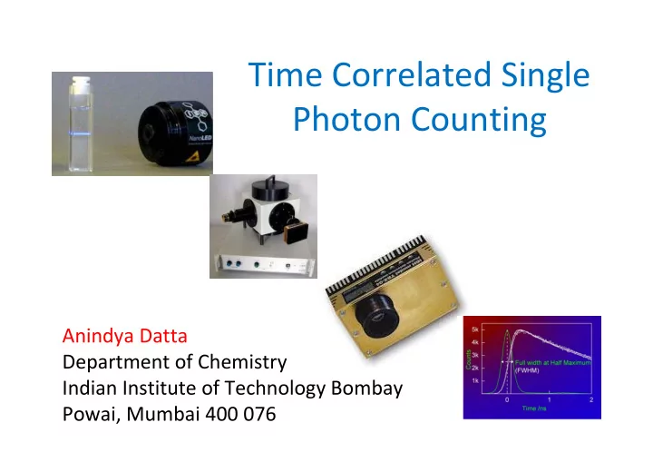
Time Correlated Single Photon Counting Anindya Datta Department of - PowerPoint PPT Presentation

Time Correlated Single Photon Counting Anindya Datta Department of Chemistry Indian Institute of Technology Bombay Powai, Mumbai 400 076

Fluorescence Decay Following Pulsed Excitation        t  * * N t N 0 exp       * F t N t        t   F t F 0 exp  Where N*(t) = Population of the excited state at time t F*(t) = Fluorescence intensity at time t Multiple independent decay pathways: Multiexponential decays         t   0 exp F t F a    i i

Fluorescence Lifetime and the Depopulation Rates    k R Radiative Nonradiative     1 k NR k R k NR • Window to excited state dynamics Photoisomerization, Excited State Proton Transfer, Charge Transfer, Exciplexes, Energy Transfer • Microenvironment sensitive Protein folding, Microheterogeneous media • Imaging and Microscopy

Schematics of the Instrument Sample T ime DL chamber Short Laser Pulse P C orrelated S ingle P P hoton Mono- C ounting chromator TBX-04 Delay CFD CFD Sync. Trigger PS: Power supply, P S Stop Start DL: Diode laser, P: Polariser TAC CFD: Constant fraction IBH Data Station Out discriminator TAC: Time to amplitude converter MCA: Multichannel annalyser Computer with MCA

The essence of TCSPC Sample DL chamber Short Laser Pulse P P Mono- chromator TBX-04 Delay CFD CFD Sync. Trigger P S Stop Start TAC IBH Data Station Out • TAC range: Time for which TAC waits for a STOP Computer with MCA • Number of channels

Constant Fraction Discrimination Sample DL chamber Short Laser Pulse P P Mono- chromator TBX-04 Delay CFD CFD Sync. Trigger P S Stop Start TAC IBH Data Station Out Computer with MCA Timing jitter = 50 ps for CFD, 1 ns for LED

Data Analysis: Iterative Reconvolution Finite pulse width:   F L F Convolution D           F t F t t ' P t ' dt ' D 0 P(t ′ ) = Impulse function at time t ′ F(t ‐ t ′ ) = Intensity at time t, from Exponential decay with origin at time t ′   Range of t ′ = Determined by shape of pulse      t  * * N t N 0 exp       * F t N t        t   F t F 0 exp 

Data Analysis: Iterative Reconvolution

Data Analysis: Iterative Reconvolution           F t F t t ' P t ' dt ' D P(t’) 0 F(t ‐ t’)P(t’) t ‐ t’ t’ t

Data Analysis: Iterative Reconvolution           F t F t t ' P t ' dt ' D 0 t The Guess Fitting Function is Convoluted with the Instrument Response Function and the Function thus generated is compared with the observed Decay

Goodness of Fit Reduced χ 2 :      F   2    2   i  Y i D i  1 Y ( i )     N  p  i     N Y(i) = Experimentally obtained data at point no. i F D (i) = Fitting data after convolution N = Number of data points. P = Number of parameters Reduced χ 2 should be equal to 1 for a good fit    F      Y i D i R i Weighted Residuals:    i Deviation at each point can be determined  2     2 R i i

Global analysis of TCSPC data Steady State Spectrum Global  2 = Average value of local  2 Intensity 3 ns 7 ns Wavelength Local Parameters Depend on wavelength             t t     F t F 0 a exp a exp          1 2  1 2 3 ns 7 ns Global parameters Wavelength independent

Life beyond Multiexponential decays Heterogeneous environments • Distribution of lifetimes • Stretched exponential function I(t ) = I 0 exp( ‐ t/ τ ) β  provides a measure of heterogeneity Rouvière N, Gallay J. 2000. Cell Mol Biol 46(5):1113–1131.

Time resolved emission spectra Steady State Spectrum Multiexponential decay TCSPC Intensity I ss ( λ′ ) I ss ( λ ) a i and  i Wavelength t’ TRES Area Normalize 0 t’ t Intensity Intensity time 0 Wavelength Wavelength Isoemissive point: Two state process J. Chem. Phys. 2001 , 115 , 7094; J. Phys. Chem. A 2001 , 105 , 1767 14