Statistics, Probability, Distributions, & Error Propagation - PowerPoint PPT Presentation
Statistics, Probability, Distributions, & Error Propagation James R. Graham 9/2/09 1 Sample & Parent Populations Make measurements x 1 x 2 In general do not expect x 1 = x 2 But as you take more and more
Statistics, Probability, Distributions, & Error Propagation James R. Graham 9/2/09 1
Sample & Parent Populations • Make measurements – x 1 – x 2 – In general do not expect x 1 = x 2 – But as you take more and more measurements a pattern emerges in this sample • With an infinite sample x i , i ∈ {1… ∞ } we can – Expect a pattern to emerge with a characteristic value – Exactly specify the distribution of x i – The hypothetical pool of all possible measurements is the parent population – Any finite sequence is the sample population 2
Histograms & Distributions • Histogram represents the occurrence or frequency of discrete measurements – Parent population (dotted) – Inferred parent distribution (solid) 3
Notation • Parent distribution: Greek, e.g., µ • Sample distribution: Latin, x – To determine properties of the parent distribution assume that the properties of the sample distribution tend to those of the parent as N tends to infinity 4
Summation • If we make N measurements, x 1 , x 2 , x 3 , etc. the sum of these measurements is N ∑ = x 1 + x 2 + x 3 + ... + x N x i i = 1 • Typically, we use the shorthand N ∑ ∑ = x i x i i = 1 5
Mean • The mean of an experimental distribution is x = 1 ∑ x i N • The mean of the parent population is defined as ⎛ ⎞ 1 ∑ µ = lim x i ⎝ ⎠ N →∞ N 6
Median • The median of the parent population µ 1/2 is the value for which half of x i < µ 1/2 P ( x i < µ 1/2 ) = P ( x i ≥ µ 1/2 ) = 1/2 • The median cuts the area under the probability distribution in half 7
Mode • The mode is the most probable value drawn from the parent distribution – The mode is the most likely value to occur in an experiment – For a symmetrical distribution the mean, median and mode are all the same 8
Deviation • The deviation, d i , of a measurement, x i , from the mean is defined as d i = x i − µ • If µ is the true mean value the deviation is the error in x i 9
Mean Deviation • The mean deviation vanishes! – Evident from the definition ⎡ ⎤ ⎡ ⎤ 1 1 ∑ ∑ N →∞ d = lim ( x i − µ ) ⎥ = lim − µ lim x i ⎢ ⎢ ⎥ ⎣ ⎦ ⎣ ⎦ N N N →∞ N →∞ µ 10
Mean Square Deviation • The mean square deviation is easy to use analytically and justified theoretically ⎡ ⎤ ⎡ ⎤ σ 2 = lim 1 ( ) 1 ∑ ∑ 2 x i − µ ⎥ = lim ⎥ − µ 2 2 x i ⎢ ⎢ ⎣ ⎦ ⎣ ⎦ N N N →∞ N →∞ • σ 2 is also known as the variance – Derive this expression – Computation of σ 2 assumes we know µ 11
Population Mean Square Deviation • The estimate of the standard deviation, s, from a sample population is s 2 = 1 ( ) ∑ 2 x i − x N − 1 • The factor ( N- 1) is used instead of N to account for the fact that the mean must be derived from the data 12
Significance • The mean of the sample is the best estimate of the mean of the parent distribution – The standard deviation, s , is characteristic of the uncertainties associated with attempts to measure µ – But what is the uncertainty in µ ? • To answer these questions we need probability distributions… 13
µ and σ of Distributions • Define µ and σ in terms of the parent probability distribution P ( x ) – Definition of P ( x ) • Limit as N → ∞ • The number of observations dN that yield values between x and x + dx is dN/N = P(x) dx 14
Expectation Values • The mean, µ , is the expectation value of some quantity x <x> • The variance, σ 2 , is the expectation value of the deviation squared <(x- µ ) 2 > 15
Expectation Values • For a discrete distribution, N , observations and n distinct outcomes N 1 ∑ µ = Lim x i N →∞ N i = 1 n 1 ∑ = Lim x j n x j each x j is a unique value N →∞ N j = 1 n 1 ∑ = Lim x j NP ( x j ) N →∞ N j = 1 n ∑ = Lim x j P ( x j ) N →∞ j = 1 16
Expectation Values • For a discrete distribution, N , observations and n distinct outcomes N σ 2 = Lim 1 ∑ ( x i − µ ) 2 N N →∞ i = 1 n 1 ∑ = Lim ( x j − µ ) 2 NP ( x j ) N N →∞ j = 1 [ ] n ∑ = Lim ( x j − µ ) 2 P ( x j ) N →∞ j = 1 17
Expectation values • The expectation value of any continuous function of x ∞ ∫ f ( x ) = f ( x ) P ( x ) dx −∞ ∞ ∫ µ = xP ( x ) dx −∞ σ 2 = ∞ ( x − µ ) 2 P ( x ) dx ∫ −∞ ∞ ∫ P ( x ) dx = 1 where −∞ 18
Binomial Distribution • Suppose we have two possible outcomes with probability p and q = 1- p – e.g., a coin toss, p = 1/2, q = 1/2 1/2 • If we flip n coins what is the probability of getting x heads? h t – Answer is given by the Binomial Distribution P ( x ; n , p ) = C ( n , x ) p x q n − x – C ( n , x) is the number of combinations of n items taken x at a time = n !/[ x !( n-x)!] 19
Binomial Distribution • The expectation value n ∑ P ( x ; n , p ) µ = x x = 0 n ∑ C ( n , x ) p x q n − x = x x = 0 ⎡ ⎤ n ∑ n ! = x !( n − x )! p x (1 − p ) n − x ⎥ = np ⎢ x ⎣ ⎦ x = 0 20
Poisson Distribution • The Poisson distribution is the limit of the Binomial distribution when µ << n because p is small – The binomial distribution describes the probability P ( x ; n, p ) of observing x events per unit time out of n possible events – Usually we don’t know n or p but we do know µ 21
Poisson Distribution • Suppose p << 1 then x << n n ! x !( n − x )! p x (1 − p ) n − x P ( x ; n , p ) = n ! ( n − x )! = n ( n − 1)( n − 2)...( n − x − 2)( n − x − 1) ≈ n x when n >> x ( n − x )! p x ≈ ( np ) x = µ x n ! (1 − p ) n − x = (1 − p ) − x (1 − p ) n ≈ 1 × (1 − p ) n since p << 1 µ = e − 1 µ = e − µ ( ) p → 0 (1 − p ) n = Lim p → 0 (1 − p ) 1/ p ⎡ ⎤ Lim ⎣ ⎦ P ( x , µ ) = µ x x ! e − µ 22
Poisson Distribution • The expectation value of x is ∞ ∞ µ x x ! e − µ = µ ∑ ∑ x = xP ( x , µ ) = x x = 0 x = 0 • Expectation value of ( x- µ ) 2 ∞ µ x 2 = σ 2 = x ! e − µ = µ ( ) ∑ x − µ ( x − µ ) 2 x = 0 23
Gaussian or Normal Distribution • The Gaussian distribution is an approximation to the binomial distribution for large n and large np 2 x − µ ⎛ ⎞ − 1 1 ⎜ ⎟ ⎝ ⎠ P ( x ; µ , σ ) = σ 2 2 π e σ 24
Gaussian or Normal Distribution 2 ⎛ ⎞ x − µ − 1 ⎜ ⎟ 1 P ( x ; µ , σ ) = ⎝ σ ⎠ 2 e σ 2 π 2 ⎛ ⎞ x − µ − 1 1 ∫ ⎜ ⎟ 1 1 − 1 2 x 2 dx = 0.683 P ( x ; µ , σ ) = ⎝ σ ⎠ e 2 e 2 π − 1 σ 2 π +/- 1 σ : 68.3% +/- 2 σ : 95.5% +/- 3 σ : 99.7% 25
Combining Two Observations • Suppose I have two sets of measurements, a i , and b i – A derived quantity c i = a i + b i – What is the relation between the means and standard deviations of a i and b i and c i – Suppose we have the same number of observations N of a i and b i 26
Combining Two Observations N = N a = N b a = 1 ∑ b = 1 ∑ a i b i N N 2 = c = 1 ∑ 1 ∑ ( ) 2 c i − c c i s c N − 1 N c i = a i + b i c = 1 ∑ b i ) = 1 ∑ 1 ∑ ( a i + a i + b i N N N = a + b 27
Combining Two Observations 2 = ∑ ( ) 2 c i − c c = a + b 1 s c , N − 1 [ ] 2 = ( ) ∑ 2 a i + b i − a + b 1 s c N − 1 [ ] 2 − 2 a i + b i ( ) + a + b ( ) ∑ ( ) ( ) a + b 2 = a i + b i 1 N − 1 [ ] 2 + b i 2 + 2 a i b i − 2 a i a + a i b + b i a + b i b ) 2 + 2 a ∑ ( ) + ( a ( ) 2 = b + b 1 a i N − 1 N − 1 a 2 + N − 1 b 2 + ) 2 − 2 N ( ) ∑ 2 = − b − N N 2 N N a i b i N − 1 ( a N − 1 a N − 1 b N − 1 28
Combining Two Observations 2 = ∑ ( ) c i − c 2 c = a + b 1 s c , N − 1 N − 1 a 2 + N − 1 b 2 + ) 2 − 2 N ( ) ∑ 2 = − b − N N 2 N N a i b i N − 1 ( a N − 1 a N − 1 b N − 1 [ ] [ ] ( ) N − 1 a 2 − ( a N − 1 b 2 − b ( ) 2 = + + 2 N N − 1 ab − a ) 2 N N b 2 2 2 s ab 2 s a s b 2 = s a 2 + s b 2 + 2 s ab 2 s c • The term s 2 ab is the covariance – Murphy’s law factor – s ab can be negative, zero or positive 29
Combining Two Uncorrelated Observations • When a and b are uncorrelated the covariance is zero 2 = ( ) ∑ ( ) b i − b a i − a = 0 1 s ab N − 1 2 = s a 2 + s b 2 s c – The variance of c is the sum of the variances of a and b • This demonstrates the fundamentals of error propagation 30
Propagation of Errors • Suppose we want to determine x which is a function of measured quantities, u , v , etc. x = f ( u , v ,...) • Assume that x = f ( u , v ,...) 31
Propagation of Errors • The uncertainty in x can be found by considering the spread of the values of x resulting from individual measurements, u i , v i , etc., x i = f ( u i , v i ,...) • In the limit of N → ∞ the variance of x 2 = Lim ∑ ( ) 2 σ x x i − x 1 N N →∞ i 32
Recommend
More recommend
Explore More Topics
Stay informed with curated content and fresh updates.

